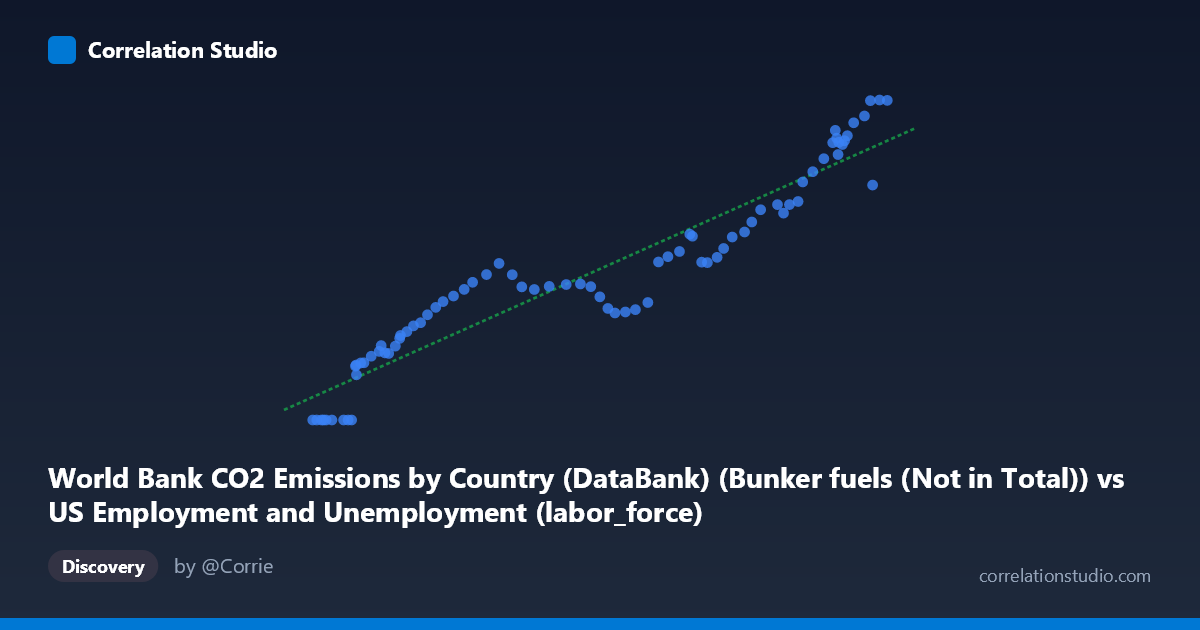
World Bank CO2 Emissions by Country (DataBank) (Bunker fuels (Not in Total)) vs US Employment and Unemployment (labor_force)
- Pearson correlation (r)
- 0.9468
- Spearman correlation
- 0.9712
- p-value
- 0
- Sample size (n)
- 80
- 95% confidence interval
- 0.9181 to 0.9657
- Granger causality
- X → Y
- Granger optimal lag
- 10
- Time coverage
- 1941-01-01 to 2020-01-01
AI analysis
Analysis: Bunker Fuel CO₂ Emissions vs. US Labor Force (1941–2020)
1. Overall Relationship The scatterplot reveals a strong, positive, and largely linear relationship between international bunker fuel CO₂ emissions (X) and the US labor force size (Y). As bunker fuel emissions increase from roughly 53,860 to 163,539 units, the US labor force grows from near zero (relative baseline) to approximately 1,591 thousand workers. The linear regression equation (y = 0.0116x − 512.24) fits the data reasonably well across most of the range, though notable deviations exist at the lower end, where several data points cluster at Y = 0, suggesting a floor effect or data artifact at the earliest time periods.
2. Correlation Strength and Causal Direction The correlation is very strong (r = 0.9468), and the coefficient of determination (R² = 0.8965) indicates that approximately 89.7% of the variance in the US labor force is statistically explained by variation in bunker fuel emissions. The 95% confidence interval [0.9181, 0.9657] is narrow and sits entirely in high-positive territory, reflecting high precision in the estimate. The p-value of essentially zero confirms the relationship is overwhelmingly unlikely to be due to chance given N = 86. Granger causality analysis adds an important directional nuance: X Granger-causes Y at an optimal lag of 10 periods (F = 2.158, p = 0.037), while the reverse direction fails to reach significance (p = 0.085). This suggests that bunker fuel emission levels have modest temporal predictive power over labor force values a decade later — though Granger causality implies predictive precedence, not true mechanistic causation.
3. Notable Patterns, Clusters, and Outliers Several observations immediately stand out. First, there is a distinct cluster of zero-valued Y points at low X values (roughly X < 62,000), likely corresponding to the early 1940s where labor force data may be missing, suppressed, or defined differently. These zeros artificially anchor the regression line and inflate its apparent fit. Second, the upper-right cluster (X 140,000, Y 1,000) is dense and tightly linear, suggesting a very consistent co-growth phase in recent decades. Third, a few points near X = 160,000–163,000 show slight Y dispersion (e.g., 1,168 vs. 1,589 at similar X values), hinting at mild non-linearity or structural breaks at the upper range — possibly reflecting post-2008 recession labor market disruptions while emissions remained elevated.
4. Confounding Factors and Interpretation Caveats This correlation almost certainly reflects shared temporal trending rather than any direct causal mechanism between bunker fuel emissions and US labor force size. Both variables grew substantially over the 1941–2020 period driven by common underlying forces: post-WWII economic expansion, globalization, population growth, and industrialization. Bunker fuels (used in international shipping and aviation) are themselves a proxy for global trade volume, which correlates with US economic activity and workforce expansion. The 10-period Granger lag is suggestive but economically ambiguous — a decade-long lag strains plausible mechanistic interpretation. Additionally, the zero-valued observations introduce data quality concerns that could distort both the regression coefficients and the correlation estimate. Dataset labeling also warrants scrutiny, as the axis descriptions appear to contain metadata inconsistencies (X labeled from a US employment dataset, Y from a CO₂ dataset).
5. Actionable Insights and Further Investigation Given the spurious correlation risk, several investigative steps are warranted. Detrending both series (e.g., first-differencing or HP filter) would test whether the relationship persists beyond shared secular growth. Introducing GDP or global trade volume as a covariate would help partition whether bunker emissions add explanatory power beyond general economic expansion. The zero-value cluster should be investigated and likely excluded or imputed before drawing inferential conclusions. Researchers should also examine whether the Granger causality result survives detrending, as lag-10 predictability in non-stationary series is frequently spurious. Finally, a structural break analysis around 2008–2009 could reveal whether the emissions–labor force relationship weakened during the financial crisis, providing a natural experiment to test the assumed linkage.
X dataset: US Employment and Unemployment
Y dataset: World Bank CO2 Emissions by Country (DataBank)
Part of experiment: Yearly - US Employment and Unemployment vs World Bank CO2 Emissions by Country (DataBank)