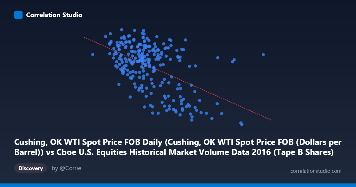
Cushing, OK WTI Spot Price FOB Daily (Cushing, OK WTI Spot Price FOB (Dollars per Barrel)) vs Cboe U.S. Equities Historical Market Volume Data 2016 (Tape B Shares)
- Pearson correlation (r)
- -0.5218
- Spearman correlation
- -0.4332
- p-value
- 0
- Sample size (n)
- 252
- 95% confidence interval
- -0.6062 to -0.4256
- Granger causality
- None
- Granger optimal lag
- 1
AI analysis
Analysis: WTI Crude Oil Prices vs. Cboe Tape B Share Volume (2016)
Relationship Overview The scatterplot reveals a negative relationship between WTI crude oil spot prices (X-axis) and Cboe Tape B share volume (Y-axis) across 252 trading days in 2016. As oil prices increase, Tape B equity share volume tends to decrease. The linear regression equation (y = -1.16169E-07x + 55.74) confirms this inverse trend, though the scatter around the regression line is substantial. This suggests that while the relationship is real and statistically meaningful, it is far from deterministic — many other forces are clearly at work simultaneously.
Correlation Strength and Statistical Significance The Pearson correlation of r = -0.5218 indicates a moderate negative association. However, the r² of 0.2722 is the more sobering figure: oil prices explain only about 27.2% of the variance in Tape B volume, leaving roughly 73% unexplained by this relationship alone. The 95% confidence interval of [-0.6062, -0.4256] is entirely negative and does not cross zero, and the p-value is effectively zero against a population of N = 3,622, confirming that this correlation is highly unlikely to be a chance artifact. That said, the Granger causality results add an important nuance: neither variable significantly predicts the other temporally (X→Y: F = 1.02, p = 0.31; Y→X: F = 1.43, p = 0.23). This means that while the two variables co-move in a cross-sectional sense, knowing yesterday's oil price does not meaningfully improve forecasts of today's Tape B volume, and vice versa. The relationship appears contemporaneous and associative rather than directionally causal.
Notable Patterns, Clusters, and Outliers Several structural features stand out in the data. There is a visible cluster of high-volume, lower-price observations (oil roughly $30–38/barrel, Tape B shares ~45–52), corresponding likely to the early 2016 period when oil was depressed and equity market activity was elevated — possibly reflecting heightened uncertainty and volatility-driven trading. Conversely, as oil prices rise toward $45–55/barrel, Tape B volume tends to compress into a tighter, lower range (~40–50 shares). A handful of outlier points appear at high oil prices ($130–170M in X-axis units) but unusually low Y values (~29–34), which deviate markedly from the central cluster and may disproportionately influence the regression slope. The relationship also appears to flatten or weaken at mid-range oil prices, hinting at potential non-linearity that a simple linear model may not fully capture.
Confounding Factors and Caveats Several important caveats apply. First, 2016 was an atypical year for oil markets — prices began near multi-year lows (~$26–30/barrel) and recovered substantially by year-end, creating a strong temporal trend that can artificially inflate correlation with any other trending variable. Second, Tape B volume (covering NYSE American-listed securities) may be influenced heavily by sector composition, particularly energy stocks, which would create a mechanical feedback loop with oil prices rather than a true independent relationship. Third, common drivers — such as macroeconomic sentiment, risk-off/risk-on positioning, Federal Reserve policy, and broad market volatility (VIX) — likely drive both variables simultaneously, making it difficult to attribute any directional influence. The absence of Granger causality reinforces that the observed correlation may largely reflect shared exposure to underlying macro conditions rather than a direct link.
Actionable Insights and Further Investigation Given the moderate correlation and lack of Granger causality, practitioners should be cautious about using oil prices as a direct trading signal for Tape B volume. However, several follow-up investigations would be valuable: (1) Introduce VIX or broader volatility measures as controls to test whether the oil–volume correlation survives after accounting for market-wide uncertainty. (2) Disaggregate Tape B volume by sector to determine whether energy-sector stocks are disproportionately driving the relationship. (3) Test for non-linear or threshold effects — for example, whether the relationship strengthens specifically during oil price crashes below $35/barrel. (4) Extend the analysis to multiple years to assess whether 2016's unique oil price recovery trajectory makes this correlation a year-specific artifact rather than a durable structural feature. (5) Consider a vector autoregression (VAR) framework with additional macro controls to more rigorously assess the conditional predictive relationship between these two series.
X dataset: Cboe U.S. Equities Historical Market Volume Data 2016
Y dataset: Cushing, OK WTI Spot Price FOB Daily
Part of experiment: Daily - Cboe U.S. Equities Historical Market Volume Data 2016 vs Cushing, OK WTI Spot Price FOB Daily