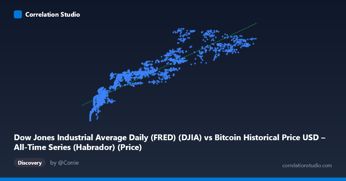
Dow Jones Industrial Average Daily (FRED) (DJIA) vs Bitcoin Historical Price USD – All-Time Series (Habrador) (Price)
- Pearson correlation (r)
- 0.9183
- Spearman correlation
- 0.9537
- p-value
- 0
- Sample size (n)
- 2390
- 95% confidence interval
- 0.9118 to 0.9243
- Granger causality
- None
- Granger optimal lag
- 10
- Time coverage
- 2016-10-24 to 2026-04-28
- Recomputed on refreshed data
- 2026-10-23 (r was 0.9183)
AI analysis
Analysis: DJIA vs. Bitcoin Price Relationship
1. What the Visualization Reveals
The scatterplot shows a strong positive relationship between the Dow Jones Industrial Average (X) and Bitcoin's historical price (Y), but the shape of the relationship is notably non-linear, resembling a logarithmic or concave curve rather than a straight line. At low DJIA values (roughly under 20,000), Y (Bitcoin) rises steeply — moving from ~18,000 to ~30,000 as X moves from ~500 to ~15,000. Beyond that point, the curve flattens considerably, with Y climbing much more slowly (from ~35,000 to ~50,000) even as X ranges from 30,000 all the way to 124,720. This pattern suggests the linear correlation coefficient, while high, is masking curvature in the actual relationship.
2. Strength, Direction, and Statistical Confidence
The Pearson correlation of r = 0.9153 indicates a strong positive linear association, and r² = 0.8377 means the linear model explains about 84% of the variance in Y — a substantial figure, though it likely overstates the fit quality given the visible curvature (a log or power transform of X would likely push explained variance even higher). The tight confidence interval [0.9087, 0.9214] and p ≈ 0 confirm this correlation is highly stable and not a product of sampling noise, given the large n (2,493).
However, the Granger causality results are the critical caveat: neither direction (X→Y or Y→X) shows significant predictive causality (p = 0.126 and p = 0.419, respectively, at 10 lags). This means that despite the strong contemporaneous correlation, neither series reliably predicts the other's future movements in a time-series sense. The relationship is best understood as co-movement rather than one variable driving the other.
3. Notable Patterns and Outliers
The data shows a clear compression/saturation effect at high X values — multiple points with very different DJIA values (e.g., X≈69,455 vs. X≈124,720) produce similar Y values in the 40,000–50,000 range, indicating diminishing marginal association. There's also a visible dense cluster at low X (under 15,000) where Y varies relatively little (18,000–30,000), suggesting this region behaves almost like a distinct regime compared to the more dispersed higher-X region. Points like (88,607, 48,362) and (72,770, 48,739) suggest a possible plateau or ceiling effect in Y, or alternatively increased variance/noise at high X.
4. Confounding Factors and Caveats
This is a classic case of spurious correlation risk driven by shared temporal trends. Both DJIA and Bitcoin prices have exhibited long-term upward trajectories over the 2016–2026 window due to macroeconomic conditions (low interest rates, monetary expansion, inflation, speculative capital flows) rather than any direct causal mechanism linking them. The lack of Granger causality strongly supports this interpretation — the correlation is likely an artifact of both series independently trending upward over time (non-stationarity), rather than evidence of a genuine economic relationship. Additionally, Bitcoin's price is denominated in USD and influenced by crypto-specific factors (halving cycles, regulatory news, exchange dynamics) that are unrelated to equity markets.
5. Actionable Insights and Further Investigation
- Detrend or difference both series (e.g., use daily/monthly returns instead of price levels) and recompute correlation — this is essential to test whether the relationship survives after removing shared time trends, which is likely the primary driver here. - Test for cointegration (e.g., Engle-Granger or Johansen test) rather than relying on simple correlation, since both series appear non-stationary. - Apply a log or power transformation to X given the visible curvature, and refit the regression — this will likely improve model fit and better reflect the true functional form. - Segment the analysis by time period (e.g., pre/post 2020, pre/post major Bitcoin halvings) to check if the relationship is stable or driven by specific market regimes (e.g., COVID-era stimulus). - Treat this correlation as descriptive, not predictive or causal — given the Granger results, it should not be used for forecasting one asset from the other.
X dataset: Bitcoin Historical Price USD – All-Time Series (Habrador)
Y dataset: Dow Jones Industrial Average Daily (FRED)
Part of experiment: Bitcoin - Bitcoin Historical Price USD – All-Time Series (Habrador) vs Dow Jones Industrial Average Daily (FRED)