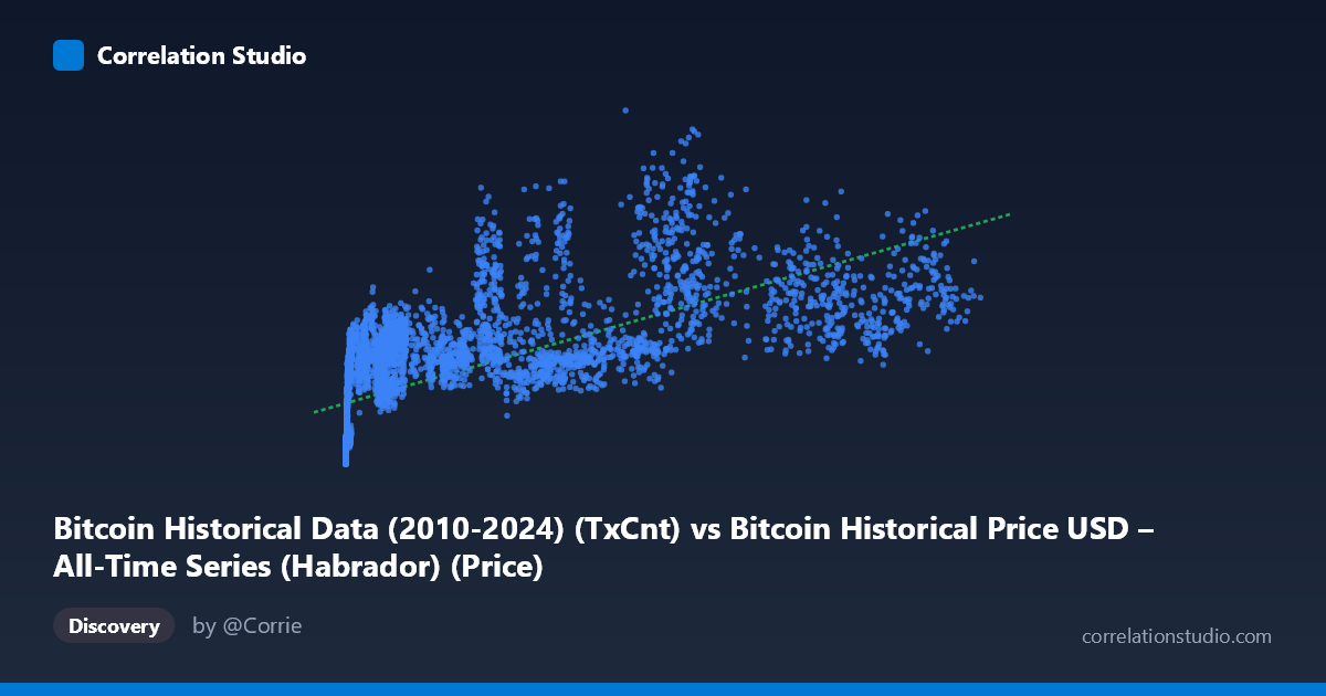
Bitcoin Historical Data (2010-2024) (TxCnt) vs Bitcoin Historical Price USD – All-Time Series (Habrador) (Price)
- Pearson correlation (r)
- 0.673
- Spearman correlation
- 0.8701
- p-value
- 0
- Sample size (n)
- 5764
- 95% confidence interval
- 0.6586 to 0.6869
- Granger causality
- None
- Granger optimal lag
- 10
AI analysis
Analysis: Bitcoin Transaction Count vs. Price
1. What the Visualization Reveals
The scatterplot shows a positive but noisy relationship between Bitcoin's daily transaction count (X) and its USD price (Y). Rather than a tight linear band, the data forms a broad, fan-shaped cloud — at low transaction counts (under ~1,000), prices cluster tightly near zero (hundreds to low thousands of dollars), while at higher transaction counts (10,000–120,000+), prices scatter widely across a huge range ($200,000–$900,000+). This heteroscedastic pattern (variance increasing with X) is a strong visual cue that a simple linear model is not fully capturing the underlying dynamics.
2. Strength, Direction, and Uncertainty
The Pearson correlation (r = 0.673) indicates a moderate-to-strong positive relationship, but r² = 0.453 tells the more important story: only 45% of the variance in price is explained by transaction count, leaving over half unexplained by this single variable. The 95% CI [0.659, 0.687] is narrow, and p ≈ 0 confirms this correlation is highly statistically significant and not a product of chance — unsurprising given n = 5,764. However, statistical significance here reflects the large sample size more than practical predictive power, since r² remains moderate.
Critically, the Granger causality tests show no significant predictive direction in either direction (X→Y: p = 0.994; Y→X: p = 0.369). This means neither past transaction counts reliably predict future price movements, nor vice versa, at the tested lag structure. This is an important caveat: despite the contemporaneous correlation, there's no evidence of a temporal, lead-lag relationship — the two series may be moving together due to a shared underlying driver (e.g., overall market growth/adoption cycles) rather than one causing the other.
3. Notable Patterns and Non-linear Features
Several features stand out: - Non-linear shape: The note that Spearman ρ exceeds Pearson r is a strong signal — the relationship is likely monotonic but curved (logarithmic or power-law), consistent with Bitcoin's known behavior where price grows multiplicatively while transaction counts grow more incrementally. - Fan/cone pattern: Variance in Y balloons as X increases, suggesting a multiplicative rather than additive relationship — a log-log transformation would likely linearize this substantially. - Clustering by market cycle: Points like (26930, 626942) and (58303, 656568) reveal that similar transaction counts can correspond to wildly different prices — this reflects Bitcoin's multi-year bull/bear cycles (2013, 2017, 2021 halvings/bubbles) where price detached from network usage during speculative peaks. - Low-X outliers with elevated Y: Points like (429, 222012) or (798, 294641) show high prices despite very low transaction counts — likely from later years (e.g., 2023-24) when fees/priorities shifted transaction economics, or from periods where large-value transfers occurred without high transaction volume.
4. Confounding Factors and Caveats
The most significant confound is time itself. Both transaction count and price have grown secularly over Bitcoin's 2010–2026 history, so much of the correlation may simply reflect two series that both trend upward over 15+ years rather than a direct causal link. This is a classic spurious correlation via shared time trend risk. Other confounders include: - Halving cycles affecting scarcity/price independent of usage - Speculative bubbles (2017, 2021) that decoupled price from fundamentals/network activity - Changing on-chain behavior (batching, SegWit, Lightning Network adoption post-2018) that reduces transaction counts per unit of economic activity over time, breaking any stable X-Y mapping - Exogenous macro factors (interest rates, regulatory news, institutional adoption) driving price independent of network fundamentals
5. Actionable Next Steps
1. Detrend or difference both series (or use log returns) to test whether the correlation survives after removing the shared time trend — this will clarify if the relationship is genuine or an artifact of co-trending. 2. Fit log-log or polynomial regression given the Spearman/Pearson divergence; a power-law model (Y ~ X^b) likely fits better than the linear model reported (R² = 0.453). 3. Segment by market era (pre-2017, 2017–2020, 2021+) to check for regime-dependent relationships, since network maturity and speculative dynamics likely shifted the X-Y mapping over time. 4. Incorporate additional covariates (active addresses, market cap, macro variables) in a multivariate model, since transaction count alone explains under half of price variance. 5. Given the null Granger result, avoid using transaction count as a standalone leading indicator for price forecasting; instead, treat both as co-moving symptoms of broader adoption/sentiment cycles requiring a common driving factor to be identified.
X dataset: Bitcoin Historical Price USD – All-Time Series (Habrador)
Y dataset: Bitcoin Historical Data (2010-2024)
Part of experiment: Bitcoin - Bitcoin Historical Price USD – All-Time Series (Habrador) vs Bitcoin Historical Data (2010-2024)