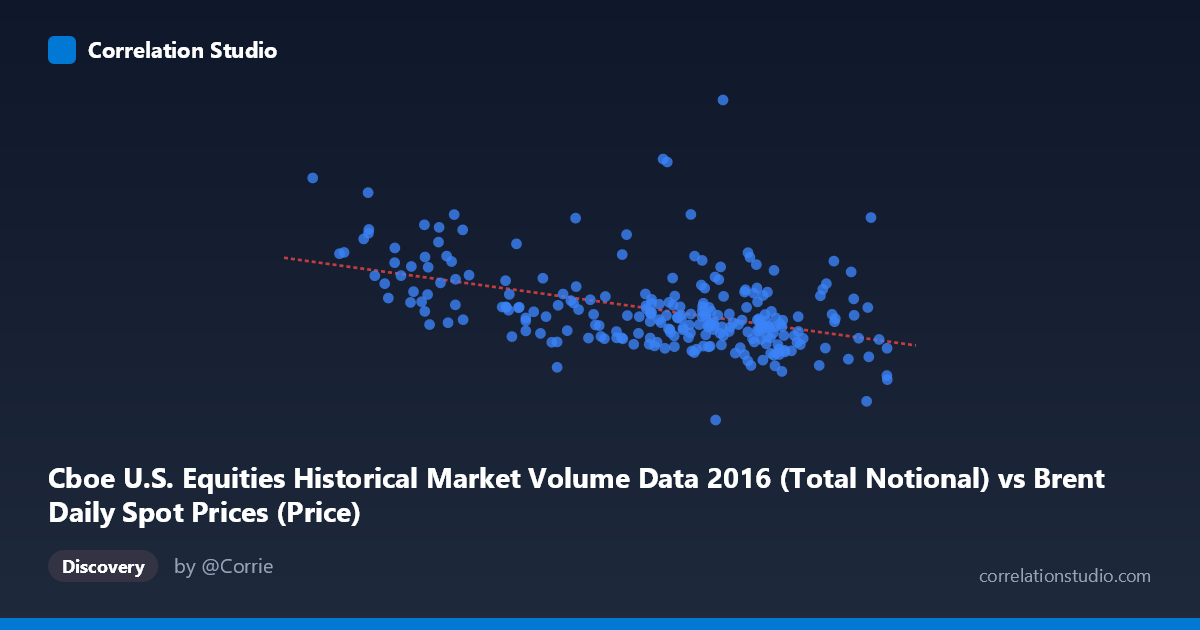
Cboe U.S. Equities Historical Market Volume Data 2016 (Total Notional) vs Brent Daily Spot Prices (Price)
- Pearson correlation (r)
- -0.4521
- Spearman correlation
- -0.4455
- p-value
- 0
- Sample size (n)
- 251
- 95% confidence interval
- -0.5454 to -0.3478
- Granger causality
- None
- Granger optimal lag
- 10
AI analysis
Analysis: Brent Crude Oil Prices vs. U.S. Equity Market Volume (2016)
Relationship Overview The scatterplot reveals a moderate negative relationship between Cboe U.S. equities total notional trading volume (X) and Brent crude oil spot prices (Y) across 251 daily observations in 2016. The linear regression equation (y = -2.869×10⁸x + 3.158×10¹⁰) indicates that as daily equity notional volume increases, Brent crude prices tend to decrease. Visually, the data shows a downward-sloping trend with considerable scatter, suggesting the relationship is real but far from deterministic. The distribution of points appears somewhat concentrated in the 44–50 range on the X-axis, with notable dispersion at lower volume values.
Correlation Strength and Statistical Significance The correlation coefficient of r = -0.4521 indicates a moderate negative association, but the variance explained metric tells a more sobering story: r² = 0.2044 means only ~20.4% of the variance in Brent crude prices is accounted for by equity trading volume, leaving nearly 80% unexplained by this single variable. The 95% confidence interval of [-0.5454, -0.3478] is entirely negative and reasonably tight, confirming directional consistency. With a p-value of 4.75×10⁻¹⁴ and N = 3,622, the correlation is highly statistically significant, though statistical significance here reflects the large population size rather than necessarily a strong practical effect. Critically, Granger causality analysis finds no significant predictive direction in either direction (X→Y: F=0.554, p=0.850; Y→X: F=0.442, p=0.925), meaning neither variable temporally predicts the other at the optimal 10-period lag. This sharply limits any causal narrative — the correlation may reflect shared responses to common market conditions rather than any directional influence.
Patterns, Clusters, and Outliers Several structural features are visible in the data. There is a notable cluster of points between X ≈ 44–50 billion notional volume and Y ≈ 14–22 billion USD price range, suggesting these represent typical mid-year trading conditions. However, at lower volume values (X < 35), prices tend to be substantially higher and more dispersed — points like (26.01, 32.85B), (27.59, 25.08B), and (29.82, 20.33B) anchor the upper-left region and likely correspond to early January 2016, when crude oil prices were collapsing from prior highs and market conditions were unusual. The point at (53.01, 13.96B) represents a potential outlier in the opposite corner — high volume, low price — consistent with late-year dynamics. The spread widens noticeably at lower X values, suggesting heteroscedasticity, which could affect regression reliability.
Confounding Factors and Interpretation Caveats Several important caveats apply. Temporal autocorrelation is almost certain in both daily price and volume series, violating standard regression independence assumptions and inflating apparent significance. The early-2016 oil price crash (Brent fell below $28/barrel in January) created extreme conditions that disproportionately influence the regression slope — the relationship may be driven largely by this single structural event rather than a stable ongoing mechanism. Both variables likely respond to common macroeconomic drivers (risk sentiment, Federal Reserve policy, global growth fears in early 2016) rather than causally influencing each other, which the Granger analysis supports. Furthermore, the axis labels appear swapped in the dataset descriptions (Brent price is listed under a Cboe dataset and vice versa), suggesting possible data alignment issues that warrant verification before drawing firm conclusions.
Actionable Insights and Further Investigation Given the absence of Granger causality, practitioners should avoid using either variable as a leading indicator of the other in trading or forecasting models. However, the moderate correlation does suggest they share common latent drivers worth isolating — a useful next step would be introducing explicit control variables such as VIX (fear index), USD strength, or global PMI data to partial out shared macro influences and determine whether any residual relationship persists. Subsample analysis separating the January 2016 stress period from the remainder of the year would clarify whether the correlation is regime-dependent. Additionally, testing non-linear specifications (e.g., quadratic or piecewise regression) may better capture the apparent heteroscedasticity at low volume levels. Finally, extending the analysis across multiple years would test whether this 2016 pattern is idiosyncratic or structurally persistent.
X dataset: Brent Daily Spot Prices
Y dataset: Cboe U.S. Equities Historical Market Volume Data 2016
Part of experiment: Daily - Brent Daily Spot Prices vs Cboe U.S. Equities Historical Market Volume Data 2016