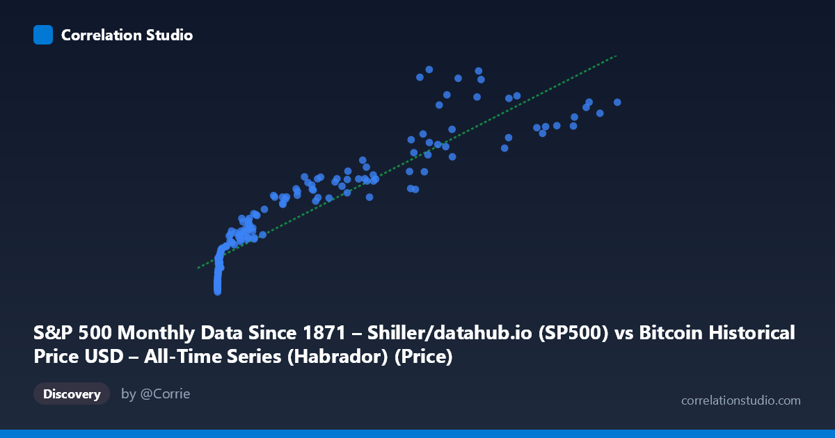
S&P 500 Monthly Data Since 1871 – Shiller/datahub.io (SP500) vs Bitcoin Historical Price USD – All-Time Series (Habrador) (Price)
- Pearson correlation (r)
- 0.9251
- Spearman correlation
- 0.9806
- p-value
- 0
- Sample size (n)
- 189
- 95% confidence interval
- 0.9014 to 0.9433
- Granger causality
- None
- Granger optimal lag
- 10
AI analysis
Analysis: Bitcoin Price vs. S&P 500 Relationship
1. What the Visualization Reveals
The scatterplot shows a strong, positive monotonic relationship between Bitcoin's historical price (X) and S&P 500 levels (Y), but the shape is distinctly non-linear. Data points cluster heavily at low X values (hundreds of points with Bitcoin under $1,000 correspond to S&P values in the 1,100–2,100 range), then stretch out into a long tail as Bitcoin climbs into the tens of thousands. This pattern is classic for a logarithmic or power-law relationship rather than a straight line — the swift, compressed rise of Bitcoin from cents to thousands of dollars matches a relatively narrow band of S&P values, while Bitcoin's later parabolic moves (to 60k, 100k+) track a further-elevated but comparatively compressed range of S&P values (5,000–7,000).
2. Strength, Direction, and Uncertainty
The Pearson correlation (r = 0.925, r² = 0.856) indicates a very strong positive linear association, with 85.6% of the variance in S&P 500 values statistically explained by Bitcoin price under a linear model. The 95% CI [0.901, 0.943] is tight, and the p-value of ~0 confirms this correlation is highly unlikely to be due to chance given the sample. However, correlation strength should not be conflated with causation or predictive power: the Granger causality tests show no significant directional predictability in either direction (X→Y: p=0.73; Y→X: p=0.59) at the optimal lag of 10 periods. This is a critical caveat — despite the strong contemporaneous statistical association, neither series helps forecast the other's future movements based on past values. This strongly suggests both variables are responding to a shared external driver (e.g., time itself, macro liquidity conditions, risk appetite) rather than one causing the other.
3. Notable Patterns and Outliers
Several features stand out: - Dense low-X cluster: The vast majority of points sit below X=1,000 with Y compressed between 1,100–2,300, reflecting Bitcoin's early years (2010–2016) when its price barely registered while the S&P moved through its own independent recovery/growth cycle. - Sparse high-X tail: Points above X=50,000 are few but show S&P values plateauing/oscillating between 4,000–7,000, suggesting the relationship flattens or becomes noisier at Bitcoin's price extremes (2021–2025 era). - Local non-monotonic wobble: Around X≈45,000, Y dips to 3,910 despite similar or lower X values elsewhere showing higher Y (e.g., X≈41,870, Y=4,454) — indicating cycle-specific divergence, likely tied to Bitcoin's crash/correction periods (2022) when equities didn't fall in the same proportion. - Compression in high-X region: The linear fit likely underestimates Y at very low X and overestimates the tightness of fit at high X, consistent with the log-like curvature visible in the scatter.
4. Confounding Factors and Caveats
The most important caveat is that both series are trending time series, and the shared time dimension (2010–2026) is almost certainly the dominant confound. Both Bitcoin and the S&P 500 have exhibited secular uptrends over this period driven by different but overlapping macro forces (post-2008 recovery, quantitative easing, low interest rates, retail investment growth, inflation hedging narratives, etc.). A spurious correlation from mutual trending is a serious risk — this is a textbook case where detrending or differencing the series (e.g., using returns instead of levels) would give a more honest picture of co-movement. Additionally, the sample (n=189) is drawn from a much larger population (N=1,865), and monthly aggregation may mask short-term volatility clustering unique to Bitcoin that doesn't exist in the S&P.
5. Actionable Insights and Further Investigation
- Do not use this correlation for trading/forecasting purposes — the lack of Granger causality confirms that neither series leads the other in a predictively useful way. - Re-run correlation on log-transformed X and/or returns (month-over-month % change) rather than raw levels to test whether the relationship holds after removing shared trend/scale effects — this is the single most important next step. - Test for cointegration (e.g., Johansen or Engle-Granger tests) to determine if there's a genuine long-run equilibrium relationship despite no Granger causality in levels. - Segment by market regime (e.g., pre-2017, 2017–2021, 2021+) to see if the correlation strength or shape changes across Bitcoin's distinct boom/bust cycles, which the wobble around X≈45,000 hints at. - Introduce a third variable (e.g., Fed funds rate, M2 money supply, or VIX) to test whether it better explains the shared movement, since the current model likely reflects confounded macro liquidity trends rather than a direct economic linkage between crypto and equities.
X dataset: Bitcoin Historical Price USD – All-Time Series (Habrador)
Y dataset: S&P 500 Monthly Data Since 1871 – Shiller/datahub.io
Part of experiment: Bitcoin - Bitcoin Historical Price USD – All-Time Series (Habrador) vs S&P 500 Monthly Data Since 1871 – Shiller/datahub.io