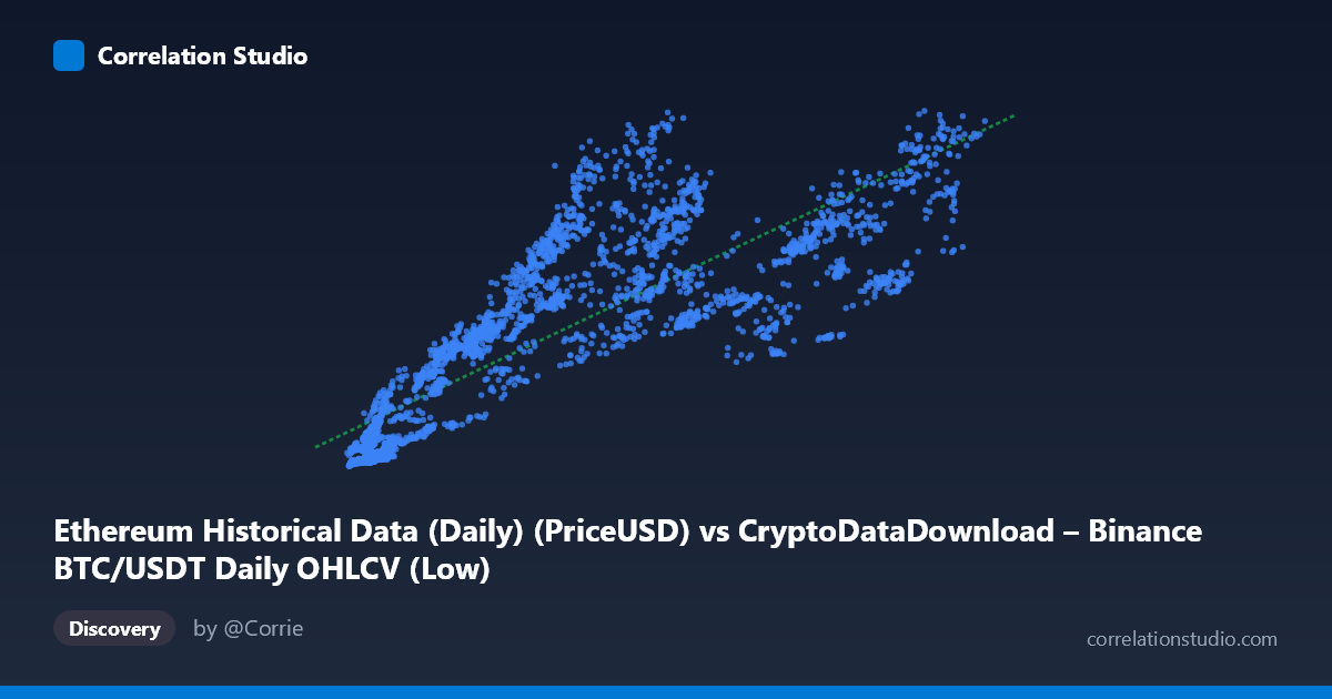
Ethereum Historical Data (Daily) (PriceUSD) vs CryptoDataDownload – Binance BTC/USDT Daily OHLCV (Low)
- Pearson correlation (r)
- 0.8386
- Spearman correlation
- 0.9076
- p-value
- 0
- Sample size (n)
- 3191
- 95% confidence interval
- 0.828 to 0.8486
- Granger causality
- None
- Granger optimal lag
- 5
- Time coverage
- 2017-08-17 to 2026-05-20
AI analysis
Analysis of the Scatterplot Relationship
1. Overview of the Relationship
The scatterplot displays a clear positive association between the X-axis variable (labeled as Ethereum PriceUSD, though this is likely a mislabeled column given the context describes BTC/USDT OHLCV data) and Y-axis variable (labeled as the "Low" price). As X increases from roughly 2,800 to 123,000, Y rises correspondingly from under 100 to nearly 4,800. The sample points confirm a generally upward-sloping pattern, though with meaningful scatter — the relationship is far from a tight linear band.
2. Strength, Direction, and Statistical Confidence
The correlation coefficient (r = 0.8386) indicates a strong positive linear relationship. However, r² = 0.7033 tells the more practically important story: only about 70% of the variance in Y is explained by X, leaving 30% unexplained by this simple linear model. The 95% confidence interval [0.828, 0.849] is tight, reflecting the large sample size (n=3,191) and giving high confidence that the true population correlation is genuinely in this strong-but-not-perfect range. The p-value of ~0 confirms this correlation is highly statistically significant and not due to chance.
Critically, the Granger causality results show no significant predictive direction in either direction (X→Y: p=0.283; Y→X: p=0.552). This is an important caveat: despite the strong contemporaneous correlation, neither variable helps forecast the other's future values based on past values at the tested lag (5 periods). This suggests the relationship is likely driven by a shared underlying factor (such as overall crypto market sentiment, liquidity cycles, or macroeconomic conditions) rather than one asset mechanically leading or causing movements in the other.
3. Notable Patterns and Features
Several non-linear characteristics are visible in the sample data: - Heteroscedasticity: Variance in Y increases substantially as X increases. At low X values (~4,000-10,000), Y is tightly clustered (150-450 range), but at high X values (~80,000-110,000), Y spreads widely (1,500-4,800). - Divergent low-X cluster: Some points with small X (e.g., X≈9,900, Y≈1,052; X≈8,083, Y≈705; X≈12,569, Y≈1,362) show unusually high Y relative to neighboring points, suggesting a distinct regime or time period where the ratio between variables was elevated — possibly an early market phase with different dynamics. - Compression at high X: Points like (81,659, 1,813) and (78,970, 1,566) show lower Y than expected given the trend, while (109,977, 4,277) is much higher — indicating variable Y/X ratios across the price cycle, consistent with two assets that don't move in lockstep proportion.
4. Confounding Factors and Caveats
Several caveats are essential for correct interpretation: - Column mislabeling: The metadata is confusing — X is labeled "Ethereum...PriceUSD" but its dataset description references BTC/USDT, while Y is labeled from the BTC dataset but its description discusses Ethereum network metrics. This suggests a data pipeline/labeling error that should be resolved before drawing asset-specific conclusions. - Common market-wide drivers: BTC and ETH (and crypto markets generally) are known to be highly correlated due to shared macro drivers (risk sentiment, dollar liquidity, regulatory news, exchange flows), not because one price causes the other. The lack of Granger causality supports this "co-movement without causation" interpretation. - Non-stationarity: Cryptocurrency prices are highly non-stationary (trending, volatile) over 2017-2026. Standard correlation/regression on non-stationary time series can produce spurious or inflated relationships; differencing or log-returns analysis would be more appropriate. - Time-aggregation: Daily granularity over ~9 years spans multiple bull/bear cycles, meaning the "relationship" may not be stable — it likely varies by market regime (bull run vs. bear market vs. crab market).
5. Actionable Insights and Next Steps
1. Verify data labeling — confirm which variable is actually BTC and which is ETH before publishing conclusions; the dataset descriptions contradict the column names. 2. Use returns, not levels — re-run correlation and Granger tests on log-returns or percentage changes rather than raw price levels to avoid spurious correlation from shared trends/non-stationarity. 3. Segment by market regime — split data into bull/bear/sideways periods to see if the r² and slope are stable or regime-dependent (the heteroscedasticity suggests they are not). 4. Test for a common factor — since neither Granger-causes the other, consider a third variable (e.g., BTC dominance, USD liquidity index, or a market-cap-weighted crypto index) as the true driver, and test cointegration (Johansen/Engle-Granger) rather than simple correlation. 5. Investigate the low-X outlier cluster — the anomalous points (e.g., X≈8,000-13,000 with disproportionately high Y) may correspond to a specific early time period worth isolating for separate analysis.
X dataset: CryptoDataDownload – Binance BTC/USDT Daily OHLCV
Y dataset: Ethereum Historical Data (Daily)
Part of experiment: Bitcoin - CryptoDataDownload – Binance BTC/USDT Daily OHLCV vs Ethereum Historical Data (Daily)