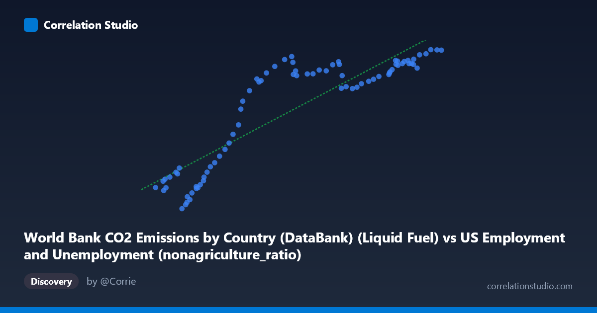
World Bank CO2 Emissions by Country (DataBank) (Liquid Fuel) vs US Employment and Unemployment (nonagriculture_ratio)
- Pearson correlation (r)
- 0.8853
- Spearman correlation
- 0.8755
- p-value
- 0
- Sample size (n)
- 80
- 95% confidence interval
- 0.8264 to 0.9251
- Granger causality
- None
- Granger optimal lag
- 10
AI analysis
Scatterplot Analysis: World Bank CO2 Liquid Fuel Emissions vs. US Non-Agriculture Employment Ratio
1. Overall Relationship The scatterplot reveals a strong positive association between World Bank CO2 emissions from liquid fuels and the US non-agriculture employment ratio over the period 1941–2020. As CO2 liquid fuel emissions increase (X-axis, ranging from ~41,250 to ~155,113 units), the non-agriculture employment ratio (Y-axis, ranging from ~2,497 to ~13,602) rises correspondingly. The linear regression equation y = 0.0924x + 535.07 describes this upward trend, though the relationship is notably non-linear across the full range, with a steep rise at lower X values that progressively flattens at higher values — suggesting a saturation or plateau dynamic in the upper range of emissions.
2. Correlation Strength, Direction, and Causality The Pearson correlation of r = 0.8853 indicates a strong positive relationship, and the R² = 0.7838 means that approximately 78.4% of the variance in the non-agriculture employment ratio is statistically explained by variation in liquid fuel CO2 emissions. This is a notably high explanatory share for a single predictor in macroeconomic data. The 95% confidence interval of [0.8264, 0.9251] is relatively tight and entirely positive, reinforcing that the correlation is robustly non-zero and directionally consistent across plausible sampling variation. The p-value of ~0 confirms the result is highly statistically significant. However, the Granger causality analysis complicates the narrative considerably: neither direction (X→Y: F=1.06, p=0.41; Y→X: F=0.94, p=0.51) achieves significance even at a generous threshold, meaning that — even with a 10-period optimal lag — neither variable temporally predicts the other in the Granger sense. This is a critical caveat: strong correlation does not imply temporal predictive power here.
3. Notable Patterns, Clusters, and Outliers The data display a clear two-regime structure. In the lower X range (~41,000–75,000), points are widely scattered with Y values spanning from roughly 2,500 to 10,000, producing high residual variance and a steep apparent slope. This likely corresponds to the mid-20th century period of rapid industrialization and labor market expansion. In the upper range (~100,000–155,000), the data cluster tightly in a band between Y ≈ 11,000–13,600, with much reduced spread — suggesting a ceiling or maturation effect in non-agriculture employment ratios. A few notable low-Y outliers appear in the lower-left quadrant (e.g., ~51,758, 2,497 and ~53,235, 2,775), which may correspond to wartime or early postwar labor disruptions. The point at (~45,010, 4,555) is somewhat anomalous given its low X value yet moderate Y, potentially representing an early structural shift.
4. Confounding Factors and Interpretation Caveats This correlation is almost certainly driven by a shared long-term temporal trend rather than a direct causal mechanism — both variables grew substantially across the 20th century as the US economy expanded, industrialized, and then matured. This is a textbook case of spurious correlation via common time trend: GDP growth, population growth, and post-WWII economic expansion simultaneously drove both liquid fuel consumption and labor force structural shifts. The Granger non-causality result at 10-period lags strongly supports this interpretation — neither series leads the other in a predictively useful way once lags are accounted for. Additionally, the dataset labeling warrants scrutiny: X is labeled as a CO2 emissions column from a US Employment dataset, and Y is labeled as a US employment column from a CO2 dataset, suggesting a cross-dataset join that may introduce alignment, methodological, or definitional inconsistencies. The non-linear shape also suggests that a linear model, despite its high R², may be misspecified.
5. Actionable Insights and Further Investigation Given the likely spurious nature of this correlation, the most productive next steps would involve detrending both series (e.g., first-differencing or HP filtering) before re-examining the correlation, which would test whether short-term fluctuations co-move beyond the shared trend. Researchers should also consider controlling for GDP, population, and energy intensity as explicit covariates, which would help isolate whether any residual relationship exists after removing common growth drivers. A structural break analysis around major events (1973 oil crisis, 2008 financial crisis, COVID-19) could explain the apparent regime shift visible in the upper cluster. Finally, expanding the Granger analysis to shorter lag windows (1–5 periods) and applying cointegration tests (e.g., Engle-Granger) would better characterize whether these series share a long-run equilibrium relationship, which would be theoretically meaningful even absent short-run Granger causality.
X dataset: US Employment and Unemployment
Y dataset: World Bank CO2 Emissions by Country (DataBank)
Part of experiment: Yearly - US Employment and Unemployment vs World Bank CO2 Emissions by Country (DataBank)