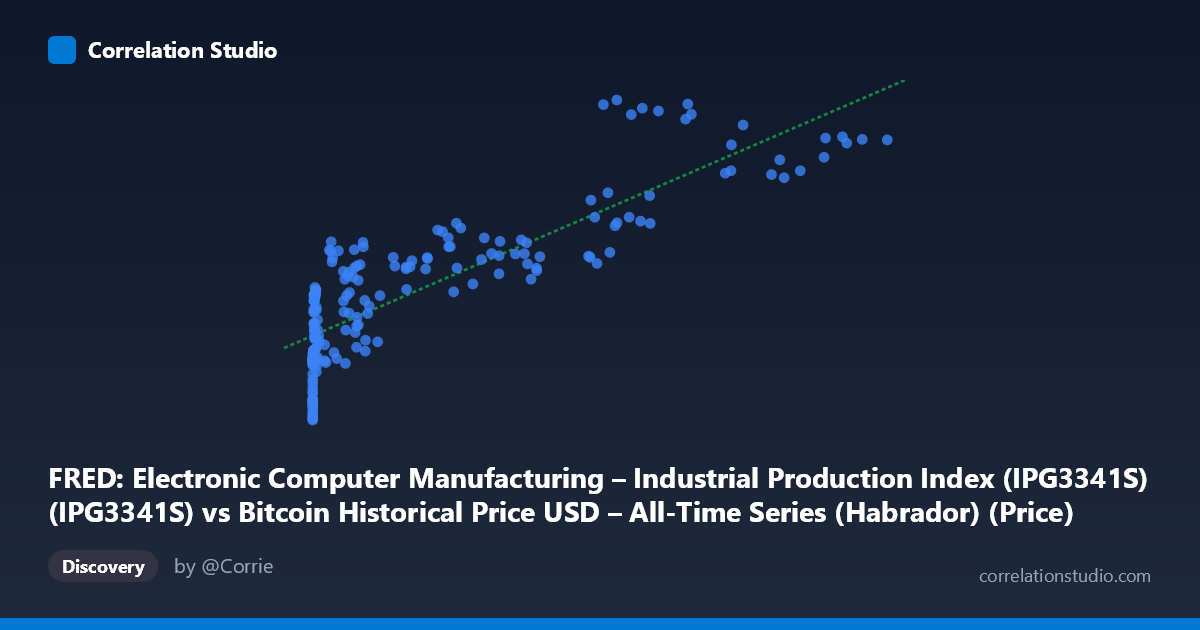
FRED: Electronic Computer Manufacturing – Industrial Production Index (IPG3341S) (IPG3341S) vs Bitcoin Historical Price USD – All-Time Series (Habrador) (Price)
- Pearson correlation (r)
- 0.8435
- Spearman correlation
- 0.8865
- p-value
- 0
- Sample size (n)
- 194
- 95% confidence interval
- 0.7974 to 0.8798
- Granger causality
- None
- Granger optimal lag
- 1
- Time coverage
- 2010-08-01 to 2026-09-01
- Recomputed on refreshed data
- 2026-10-24 (r was 0.8368)
AI analysis
Analysis: Bitcoin Price vs. Electronic Computer Manufacturing IPI
1. What the Visualization Reveals
The scatterplot shows a strong positive association between Bitcoin's historical price (X-axis) and the FRED Electronic Computer Manufacturing Industrial Production Index (Y-axis). As Bitcoin price rises across its multi-order-of-magnitude range ($0.06 to $118,670), the industrial production index climbs from roughly 75 to 181. The relationship appears non-linear in raw space—compressed near zero and spreading out at higher values—which is typical when one variable (BTC price) spans nearly 6 orders of magnitude while the other (an index) varies only ~2.4x.
2. Strength, Direction, and Statistical Confidence
The correlation coefficient (r = 0.84, R² = 0.70) indicates a strong positive linear relationship, with 70% of the variance in the computer manufacturing index statistically "explained" by Bitcoin price in this dataset. The 95% CI [0.79, 0.87] is tight and the p-value ≈ 0 confirms this correlation is not due to chance sampling noise. However, the Granger causality results are critical: neither direction shows significant predictive causality (X→Y: p=0.98; Y→X: p=0.25). This means Bitcoin price does not help forecast future values of the industrial index, nor vice versa — despite the strong contemporaneous correlation, there is no evidence of a lead-lag temporal relationship. This is a classic signature of two variables driven by a common underlying trend (e.g., time itself, or macro conditions) rather than one causing the other.
3. Notable Patterns and Outliers
The data clusters into two visible regimes: a dense low-X cluster (X < 1000, mostly early Bitcoin history, Y in the 75–120 range with high scatter) and a sparser high-X cluster (X 50,000, recent bull-market prices, Y in the 128–181 range). The low-end cluster shows considerable noise—Y values of 76–117 all crowd around X near 0–1000, indicating weak local correlation before BTC's major price appreciation. Some late points (e.g., X≈68,074 → Y=181.31, the maximum) sit above the general trend line, suggesting possible acceleration or an outlier price spike. The linear fit (R²=0.70) likely underperforms a log-transformed model given the heavy right-skew of X (mean 20,533 vs. median likely much lower, stdev 29,894).
4. Confounding Factors and Caveats
This is almost certainly a spurious or trend-driven correlation rather than a causal economic relationship. Both series have risen substantially over the 2010–2026 window: Bitcoin due to speculative adoption cycles, and the computer manufacturing index due to secular growth in semiconductor/server production (partly AI-driven in recent years). Time is the likely lurking confound — both variables trend upward over the sample period, inflating correlation. Additionally, Bitcoin price is highly volatile and event-driven (halvings, regulation, speculation), while the IPI is a slow-moving monthly industrial metric — mismatched time dynamics make genuine causality implausible. The non-Granger result reinforces that this is a level correlation (co-trending), not a functional/predictive one.
5. Suggestions for Further Investigation
- De-trend both series (e.g., using differences or growth rates rather than levels) and re-test correlation to check if the relationship survives — it likely will weaken substantially, confirming a shared-trend artifact. - Log-transform Bitcoin price given its multi-order-of-magnitude range; this may reveal a more genuine linear or saturating relationship with the index. - Consider third-variable analysis: GPU/AI hardware demand could plausibly connect crypto mining hardware needs with computer manufacturing output — investigate mining-rig demand or semiconductor shipment data as a mediating variable. - Given the lack of Granger causality, avoid using one series to forecast the other; treat this as a correlational curiosity rather than a trading or economic signal.
X dataset: Bitcoin Historical Price USD – All-Time Series (Habrador)
Y dataset: FRED: Electronic Computer Manufacturing – Industrial Production Index (IPG3341S)
Part of experiment: Bitcoin - Bitcoin Historical Price USD – All-Time Series (Habrador) vs FRED: Electronic Computer Manufacturing – Industrial Production Index (IPG3341S)