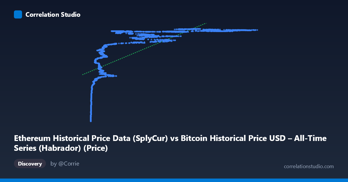
Ethereum Historical Price Data (SplyCur) vs Bitcoin Historical Price USD – All-Time Series (Habrador) (Price)
- Pearson correlation (r)
- 0.6775
- Spearman correlation
- 0.9061
- p-value
- 0
- Sample size (n)
- 3951
- 95% confidence interval
- 0.6603 to 0.6941
- Granger causality
- None
- Granger optimal lag
- 10
- Time coverage
- 2015-07-30 to 2026-05-23
- Recomputed on refreshed data
- 2026-10-24 (r was 0.6753)
AI analysis
Correlation Analysis: Ethereum Supply Metric vs. Bitcoin Historical Price
1. What the Visualization Reveals
Despite the column labels (which appear swapped or mislabeled given the dataset descriptions), the data itself shows a clear logarithmic/saturating relationship rather than a linear one. As X increases from near-zero to ~20,000, Y climbs steeply (from ~$72M to ~$120M in the sample), but beyond X≈20,000–25,000, Y plateaus and hovers in a tight band (~$119M–$121M) regardless of how high X goes (up to 124,720). This is a classic diminishing-returns/logarithmic curve shape, not a straight-line relationship.
2. Strength, Direction, and Uncertainty
The Pearson correlation (r = 0.675, R² = 0.456) indicates a moderate positive linear relationship, but this understates the true association because the underlying pattern is curved. The fact that Spearman's ρ exceeds Pearson's r confirms that a monotonic non-linear model (log or power fit) would capture substantially more of the relationship than the 45.6% variance explained by the linear model. The confidence interval [0.658, 0.692] is narrow and the p-value is effectively 0, meaning the linear correlation is highly statistically significant and precisely estimated — but statistical significance here reflects large sample size (n=3,926) more than it validates linearity as the best model.
Critically, the Granger causality test shows no significant predictive direction in either direction (X→Y: p=0.94; Y→X: p=0.82). This means neither variable helps forecast the other's future values based on past values — the correlation is likely contemporaneous/structural (both driven by shared market cycles or time trends) rather than one variable causing or leading the other. This is an important caveat: correlation coefficients describe association, not prediction, and here the data explicitly rules out lead-lag forecasting utility at the tested lag structure (up to 10 periods).
3. Notable Patterns and Features
- Compression at high X values: once X exceeds ~20,000, Y values cluster tightly near their ceiling (~120M), producing a "hockey stick" or logarithmic saturation curve. - Steep low-X region: the most dynamic, information-rich part of the relationship occurs at low X values (under 10,000), where Y ranges dramatically from ~$72M to ~$110M+. - Possible ceiling effect: Y approaching a soft cap near $121.6M (max observed) suggests either a real economic ceiling or a data-scaling/normalization artifact. - No obvious outliers breaking the pattern — the curve is smooth and consistent, suggesting genuine non-linear market dynamics rather than noise or data errors.
4. Confounding Factors and Caveats
Both series are historical price time series spanning ~11 years (2015–2026), meaning both variables are likely non-stationary and trending upward over time due to macro crypto-market growth, adoption cycles, and bull/bear phases. This shared time-trend is a classic confounder: two unrelated trending series can show spurious correlation simply because both increase over the same calendar period. The Granger non-causality result supports this concern — the relationship may be an artifact of common exposure to overall market cycles (e.g., both BTC and ETH rally/crash together due to shared sentiment, liquidity, and macro conditions) rather than a direct mechanical link. Additionally, the mislabeled column headers (Ethereum data labeled on Bitcoin's axis and vice versa) warrant a data-integrity check before drawing domain conclusions.
5. Actionable Recommendations
1. Refit with a log or power transform (e.g., log(X) vs. Y, or Box-Cox) — this will likely raise explained variance well above 45.6% and better represent the true relationship. 2. Verify column/dataset labeling — confirm which series is actually Bitcoin price and which is Ethereum price/supply before drawing economic conclusions. 3. Test for cointegration (e.g., Engle-Granger or Johansen test) rather than relying solely on Granger causality on levels — many crypto price series are cointegrated even without lead-lag predictability, especially if both are I(1) processes. 4. Detrend or difference the series (e.g., use daily returns instead of price levels) to check whether the correlation persists after removing shared time-trend effects — this will clarify whether the relationship is genuine or spurious. 5. Segment by time period (bull vs. bear market phases) to see if the correlation strength or shape changes across market regimes.
X dataset: Bitcoin Historical Price USD – All-Time Series (Habrador)
Y dataset: Ethereum Historical Price Data
Part of experiment: Bitcoin - Bitcoin Historical Price USD – All-Time Series (Habrador) vs Ethereum Historical Price Data