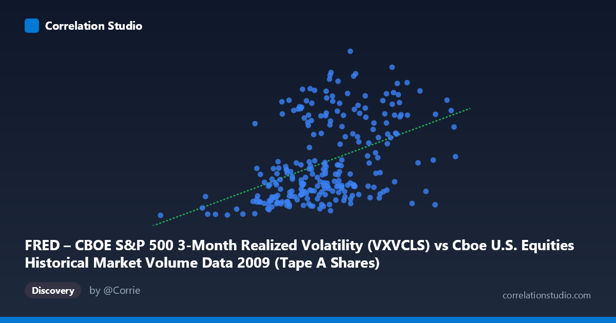
FRED – CBOE S&P 500 3-Month Realized Volatility (VXVCLS) vs Cboe U.S. Equities Historical Market Volume Data 2009 (Tape A Shares)
- Pearson correlation (r)
- 0.4428
- Spearman correlation
- 0.4687
- p-value
- 0
- Sample size (n)
- 252
- 95% confidence interval
- 0.3377 to 0.537
- Granger causality
- None
- Granger optimal lag
- 1
AI analysis
Scatterplot Analysis: CBOE S&P 500 3-Month Realized Volatility vs. Tape A Shares Volume (2009)
Relationship Overview
The scatterplot reveals a moderate positive relationship between CBOE S&P 500 3-Month Realized Volatility (VXVCLS) and Tape A Shares trading volume for U.S. equities in 2009. As realized volatility increases, Tape A share volume tends to rise as well, which is economically intuitive — periods of elevated market uncertainty typically drive heightened trading activity as investors rebalance, hedge, or react to price dislocations. The linear regression equation (y = 3.61×10⁻⁸x + 17.10) confirms this positive slope, though the relationship is far from deterministic, with considerable scatter throughout the plot space suggesting that volatility alone captures only a fraction of what drives volume.
Correlation Strength and Statistical Significance
The Pearson correlation of r = 0.4428 indicates a moderate positive association, but the coefficient of determination (R² = 0.1961) is the more sobering metric — realized volatility explains only ~19.6% of the variance in Tape A share volume, leaving roughly 80% attributable to other factors. The 95% confidence interval for r [0.3377, 0.5370] is meaningfully wide, reflecting genuine uncertainty in the precise strength of this relationship even with n = 252 paired observations drawn from a population of N = 3,232. The p-value of 1.59×10⁻¹³ confirms the correlation is highly statistically significant, making it extremely unlikely to be a chance artifact. However, Granger causality tests tell a different story temporally: neither direction (X→Y: F = 0.41, p = 0.52; Y→X: F = 0.50, p = 0.48) achieves significance at lag 1, meaning that past values of realized volatility do not reliably predict next-period volume, and vice versa. This dissociates contemporaneous correlation from predictive temporal causation — they move together, but neither leads the other.
Patterns, Clusters, and Outliers
The scatter is notably heteroscedastic: at lower volatility levels (roughly Y < 30), data points cluster tightly with relatively compressed volume ranges, while at higher volatility readings (Y 40), the spread in X values widens considerably, suggesting that high-volatility regimes produce more variable volume outcomes. There appear to be two loose clusters — a dense grouping at moderate volatility (25–35) with volumes spanning roughly 300M–550M, and a more dispersed upper cluster above 40 volatility units where volumes range widely from ~325M to over 700M. A few apparent outliers are visible at extreme coordinates: one point near (704M shares, ~34 volatility) represents unusually high volume for a moderate-volatility day, and the point near (105M shares, ~22.4 volatility) anchors the low end and may reflect a holiday-shortened or anomalous trading session in early 2009.
Confounding Factors and Caveats
Several important caveats apply. First, 2009 is a structurally unusual year — it spans the tail of the global financial crisis, a market bottom in March, and a powerful recovery rally, meaning the volatility-volume relationship may be regime-specific rather than generalizable. Second, the axes appear reversed from what the metadata labels suggest (VXVCLS on X, Tape A shares on Y), which should be verified to avoid misinterpretation. Third, realized volatility is a lagging measure by construction (3-month window), which may explain the absence of Granger causality — the signal is already "stale" relative to daily volume decisions. Fourth, confounders such as macroeconomic announcements, Fed policy actions, earnings seasons, and index rebalancing events could simultaneously drive both variables without a direct causal link between them.
Actionable Insights and Further Investigation
Practitioners should treat this correlation as suggestive context rather than a trading or operational signal — the 80% unexplained variance is too large to rely on volatility alone for volume forecasting. Recommended next steps include: (1) testing whether implied volatility (VIX) outperforms the realized VXVCLS measure in predicting volume, since implied vol is forward-looking; (2) segmenting the analysis by market regime (pre/post March 2009 bottom) to test whether the correlation strengthens in crisis versus recovery phases; (3) incorporating additional predictors (e.g., bid-ask spreads, news sentiment, options open interest) into a multivariate model to close the explanatory gap; and (4) examining longer lag structures in Granger tests (beyond lag 1) to determine whether any delayed predictive relationship emerges over weekly horizons.
X dataset: Cboe U.S. Equities Historical Market Volume Data 2009
Y dataset: FRED – CBOE S&P 500 3-Month Realized Volatility
Part of experiment: Daily - Cboe U.S. Equities Historical Market Volume Data 2009 vs FRED – CBOE S&P 500 3-Month Realized Volatility