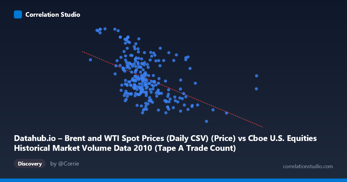
Datahub.io – Brent and WTI Spot Prices (Daily CSV) (Price) vs Cboe U.S. Equities Historical Market Volume Data 2010 (Tape A Trade Count)
- Pearson correlation (r)
- -0.468
- Spearman correlation
- -0.4619
- p-value
- 0
- Sample size (n)
- 252
- 95% confidence interval
- -0.5592 to -0.3655
- Granger causality
- None
- Granger optimal lag
- 1
AI analysis
Scatterplot Analysis: Oil Prices vs. U.S. Equity Trade Counts (2010)
Relationship Overview
The scatterplot reveals a moderate negative relationship between Brent/WTI oil spot prices (X-axis) and Cboe Tape A trade counts (Y-axis) across U.S. equity markets during 2010. As oil prices increase, equity trade counts tend to decline, with the linear regression equation y = -7.00372E-6x + 88.83 describing a gentle downward slope across the data cloud. The relationship is visually apparent but far from clean — the scatter is wide, and the trend emerges statistically rather than through an obvious visual sweep. This already signals that while a real association exists, it is embedded in considerable noise and competing influences.
Correlation Strength and Statistical Significance
The Pearson correlation of r = -0.468 indicates a moderate negative association, but the more telling figure is r² = 0.219, meaning oil prices explain only about 21.9% of the variance in equity trade counts. The remaining ~78% is driven by other factors entirely. The 95% confidence interval of [-0.559, -0.366] is reassuringly narrow given a paired sample of n = 252, and the p-value of 3.997E-15 confirms this is not a chance finding — the relationship is statistically robust across the 3,302-observation population. However, the Granger causality results are notably absent: neither direction (X→Y nor Y→X) reaches conventional significance at α = 0.05, with Y→X approaching marginal significance (F = 3.70, p = 0.056). This means that oil prices do not reliably predict next-day trade counts, and vice versa — the correlation is contemporaneous or coincidental rather than temporally predictive, which is a critical practical limitation.
Notable Patterns, Clusters, and Outliers
Several features stand out in the data. There is a loose central cluster between roughly X = 900,000–1,500,000 and Y = 74–85, where most observations concentrate. However, a distinct group of high-Y outliers (trade counts above ~88–93) appears predominantly at lower X values, suggesting elevated trading activity occurred during periods of relatively lower oil prices — potentially early 2010 or episodic volatility events. Conversely, high X values (above ~2,000,000–3,200,000) cluster tightly at lower Y values (67–77), consistent with the negative trend. The point near X = 3,216,587, Y = 76.48 and the extreme Y = 93.63 at X = 627,719 are notable outliers that may disproportionately influence the regression slope. There is also a hint of heteroscedasticity — variance in Y appears somewhat larger at lower X values — and possible non-linearity, though the linear model is a reasonable first approximation.
Confounding Factors and Interpretive Caveats
This correlation almost certainly reflects shared macroeconomic seasonality rather than a direct causal mechanism. Both oil prices and equity trading volumes are influenced by broader market risk sentiment, economic growth expectations, and calendar effects (e.g., lower volumes in summer months, higher activity around earnings seasons). The year 2010 specifically followed the 2008–2009 financial crisis and includes the May 2010 Flash Crash, which would have dramatically spiked trade counts on specific days and could distort the overall pattern. The axis labeling also deserves scrutiny — the dataset descriptions appear to cross-reference each other (Tape A counts labeled as from the oil price dataset and vice versa), which may reflect a metadata inconsistency worth verifying before drawing firm conclusions. Additionally, the negative relationship could be spurious if, for example, higher oil prices proxied for mid-year calm markets with naturally lower trading volumes.
Actionable Insights and Further Investigation
Given the moderate but statistically significant correlation and the absence of Granger causality, practitioners should avoid using oil price levels as a direct trading-volume predictor in any short-term model. However, oil prices may serve as a useful regime indicator — periods of very high or very low oil prices appear to correspond to meaningfully different trading environments. Further investigation should include: (1) controlling for VIX or market volatility to disentangle risk-sentiment confounds; (2) segmenting by sub-period (pre/post Flash Crash) to test structural stability; (3) testing non-linear models (e.g., piecewise regression or spline fitting) given the visual suggestion that the relationship may steepen at extremes; and (4) expanding to multiple years to determine whether this 2010 pattern replicates or is year-specific. A multivariate framework incorporating volatility, market returns, and macroeconomic indicators would substantially improve explanatory power beyond the current 21.9%.
X dataset: Cboe U.S. Equities Historical Market Volume Data 2010
Y dataset: Datahub.io – Brent and WTI Spot Prices (Daily CSV)
Part of experiment: Daily - Cboe U.S. Equities Historical Market Volume Data 2010 vs Datahub.io – Brent and WTI Spot Prices (Daily CSV)