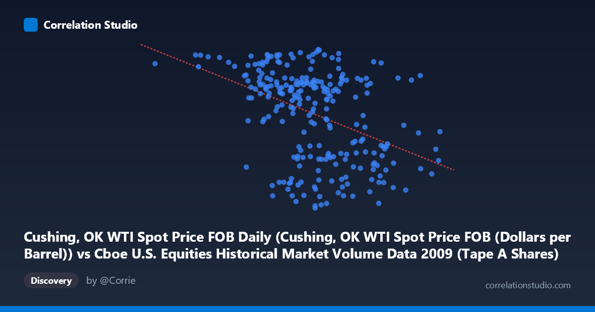
Cushing, OK WTI Spot Price FOB Daily (Cushing, OK WTI Spot Price FOB (Dollars per Barrel)) vs Cboe U.S. Equities Historical Market Volume Data 2009 (Tape A Shares)
- Pearson correlation (r)
- -0.4139
- Spearman correlation
- -0.3987
- p-value
- 0
- Sample size (n)
- 252
- 95% confidence interval
- -0.5114 to -0.306
- Granger causality
- None
- Granger optimal lag
- 1
AI analysis
Analysis: WTI Crude Oil Price vs. Cboe Equity Market Volume (2009)
Relationship Overview
The scatterplot reveals a moderate negative relationship between WTI crude oil spot prices (X-axis) and Cboe U.S. equity market share volume (Y-axis, Tape A Shares) across 252 trading days in 2009. As oil prices increase, equity trading volume tends to decline, though the relationship is far from deterministic — the data cloud is notably diffuse, with substantial vertical spread at nearly every price level. The linear regression equation (y = -5.66E-08x + 86.818) captures a downward slope, but the wide scatter makes clear that oil price alone is a poor standalone predictor of daily trading volume.
Correlation Strength and Statistical Significance
The Pearson correlation of r = -0.4139 indicates a moderate negative association. However, the r² of 0.1713 means that only ~17.1% of the variance in equity trading volume is explained by WTI prices — leaving roughly 83% attributable to other factors. While the p-value of 7.49E-12 is highly significant and the 95% confidence interval of [-0.51, -0.31] is entirely negative (confirming the directional finding is robust), statistical significance here is partly a function of the large sample (N = 3,232 population; n = 252 pairs), which inflates detection power. Critically, Granger causality tests show no significant predictive directionality in either direction — neither X→Y (F = 0.472, p = 0.493) nor Y→X (F = 0.072, p = 0.789) — meaning that past oil prices do not help forecast next-day trading volume, and vice versa. The correlation is contemporaneous and associative, not temporally predictive.
Notable Patterns, Clusters, and Outliers
Several structural features stand out in the data. There appears to be a loose clustering of high-volume observations (Y 70 billion shares) concentrated in the lower-to-mid oil price range (~$34–$55/barrel), consistent with early 2009 when markets were highly volatile post-financial crisis and oil was depressed. Conversely, at higher oil prices (~$60–$80/barrel, mid-to-late 2009), volume tends to be lower and less dispersed. A few notable outliers are visible — particularly points with very high volume at moderate oil prices and points at the extremes of the X range (e.g., the lowest oil price observation near $34–$35/barrel paired with elevated volume, and the highest price observations near $80/barrel). The relationship also shows heteroscedasticity: variance in Y appears larger at lower X values, suggesting the negative correlation may be partially driven by regime differences between early and late 2009 rather than a uniform linear mechanism.
Confounding Factors and Caveats
The observed negative correlation almost certainly reflects shared time-series dependence rather than a direct causal mechanism. In 2009, the year began with the tail end of the financial crisis (low oil prices, high market fear, elevated trading volumes driven by panic selling) and transitioned into a recovery (rising oil prices, stabilizing but normalizing volumes). This secular trend — both variables responding to a common third driver (macroeconomic recovery) — is a classic confound. Additionally, equity trading volume is influenced by volatility regimes (VIX), Federal Reserve policy actions, earnings seasons, and index rebalancing events, none of which are captured here. The axis labels also appear swapped relative to convention (the dataset description lists X as the volume data and Y as the price data), which warrants verification before drawing further conclusions.
Actionable Insights and Further Investigation
Given the lack of Granger causality, traders and analysts should not use lagged WTI prices as a signal for equity volume forecasting, nor the reverse. However, the contemporaneous correlation suggests both variables respond to common macro drivers worth modeling explicitly. Recommended next steps include: (1) introducing a volatility index (VIX) or recession indicator as a control variable to test whether the correlation disappears after accounting for the macro regime shift; (2) segmenting the data into pre- and post-crisis recovery periods (e.g., Q1 vs. Q3–Q4 2009) to test whether the correlation is regime-specific; (3) fitting a non-linear or piecewise regression to assess whether the relationship changes character at oil price thresholds; and (4) extending the time window beyond 2009 to determine if the negative correlation is a persistent structural feature or an artifact of a unique crisis year.
X dataset: Cboe U.S. Equities Historical Market Volume Data 2009
Y dataset: Cushing, OK WTI Spot Price FOB Daily
Part of experiment: Daily - Cboe U.S. Equities Historical Market Volume Data 2009 vs Cushing, OK WTI Spot Price FOB Daily