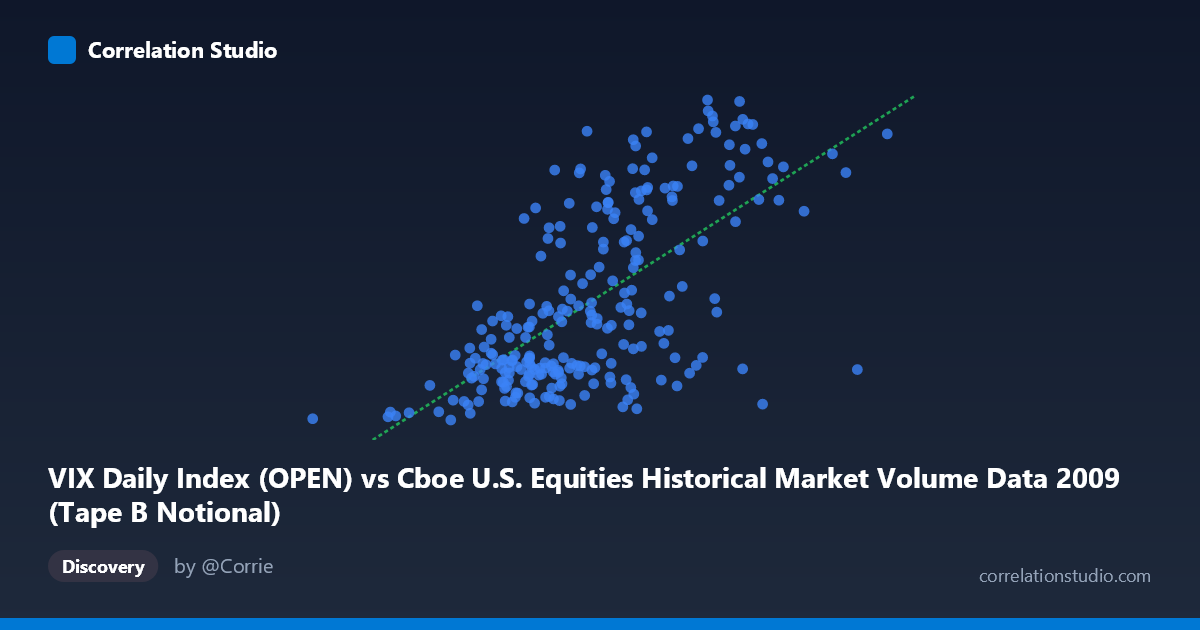
VIX Daily Index (OPEN) vs Cboe U.S. Equities Historical Market Volume Data 2009 (Tape B Notional)
- Pearson correlation (r)
- 0.6557
- Spearman correlation
- 0.6324
- p-value
- 0
- Sample size (n)
- 252
- 95% confidence interval
- 0.5791 to 0.7209
- Granger causality
- None
- Granger optimal lag
- 1
AI analysis
Scatterplot Analysis: VIX Daily Index (Open) vs. Tape B Notional Volume (2009)
Overall Relationship The scatterplot reveals a moderate positive relationship between the VIX Daily Index open values and Cboe U.S. Equities Tape B notional trading volume throughout 2009. As VIX open values increase — spanning roughly 1.3 billion to 9.5 billion on the x-axis — Tape B notional values tend to rise from approximately 19.5 to 52.65. The linear regression equation (y = 4.605×10⁻⁹x + 7.456) confirms this upward trend, suggesting that higher market volatility readings are associated with elevated notional trading activity in Tape B securities. This relationship is intuitive: periods of elevated fear or uncertainty (high VIX) historically coincide with increased trading volume as market participants reposition portfolios, execute hedges, or react to rapid price movements.
Correlation Strength and Statistical Significance The Pearson correlation of r = 0.6557 indicates a moderate-to-strong positive association, and with r² = 0.43, approximately 43% of the variance in Tape B notional volume is explained by the VIX open level — a meaningful but far from complete explanatory relationship. The remaining 57% of variance is attributable to other factors not captured here. The 95% confidence interval of [0.5791, 0.7209] is relatively tight and does not include zero, and the p-value of effectively 0 (against n = 252 paired observations drawn from a population of N = 3,232) confirms this correlation is highly statistically significant and unlikely to be a chance finding. However, the Granger causality results tell a more cautionary story: neither direction (X→Y: F = 0.040, p = 0.842; Y→X: F = 0.137, p = 0.712) reaches significance at any conventional threshold. This means that, despite a strong contemporaneous correlation, neither variable reliably predicts the other at a 1-period lag, so the relationship appears to be concurrent rather than directionally predictive in a temporal sense.
Notable Patterns, Clusters, and Outliers The scatterplot displays two visually distinct behavioral regimes rather than a smooth linear cloud. A dense cluster of points congregates at lower VIX values (roughly 1.3–5.0 billion range) with Tape B notional values tightly packed between approximately 19 and 30 — consistent with the calmer, post-crisis stabilization period in the second half of 2009. A second, more dispersed cluster occupies the upper range (VIX above 5.5 billion), where Tape B notional values spread widely from ~20 to over 52, reflecting the high-volatility, high-volume environment of early 2009 during peak financial crisis stress. Several points stand out as potential outliers — notably observations near (6.8B, 49.7), (7.5B, 50.2), and (7.3B, 50.0) — which represent extreme joint highs and may disproportionately influence the regression slope. The wide vertical spread at high X values also suggests heteroscedasticity, where variance in Y increases with X, violating a key assumption of ordinary least squares regression.
Confounding Factors and Interpretive Caveats Several important caveats temper interpretation. First, the x- and y-axis labels appear to be swapped relative to what would be expected: VIX (a volatility index) is plotted on the X-axis with values in the billions, which are atypical VIX units (VIX normally ranges ~10–80). This likely reflects that the "VIX Daily Index" dataset column being used is actually a volume or notional metric, and vice versa — suggesting a potential metadata or column-assignment error that should be verified before drawing conclusions. Second, 2009 is a highly unusual single-year window bookended by extreme crisis conditions in January and recovery by December, so the correlation may be regime-specific and not generalizable to other periods. Third, macroeconomic confounders — Federal Reserve interventions, earnings seasons, index rebalancing events, and structural market changes in 2009 — could jointly drive both variables simultaneously, producing correlation without direct causation. The absence of Granger causality reinforces this concern.
Actionable Insights and Further Investigation Practitioners should first audit the dataset column assignments to confirm which variable is genuinely VIX open and which is notional volume, as the axis scaling strongly suggests a labeling inconsistency. Assuming the relationship is real, portfolio risk managers could use elevated VIX levels as a contemporaneous signal of heightened Tape B activity, though the lack of Granger causality means it should not be used as a lead indicator for short-term trading strategies. Further investigation should include: (1) testing the relationship across multiple years to assess whether the 2009 coefficient is stable or crisis-driven; (2) applying a non-linear or regime-switching model given the apparent two-cluster structure; (3) controlling for market-wide volume trends to isolate the VIX-specific effect; and (4) examining longer optimal lags (beyond 1 period) in the Granger framework, as volatility-volume dynamics may operate on weekly rather than daily timescales.
X dataset: Cboe U.S. Equities Historical Market Volume Data 2009
Y dataset: VIX Daily Index
Part of experiment: Daily - Cboe U.S. Equities Historical Market Volume Data 2009 vs VIX Daily Index