Cboe U.S. Equities Historical Market Volume Data 2010 (Tape B Shares) vs Brent Crude Oil Prices: Daily (DCOILBRENTEU) – FRED St. Louis Fed (DCOILBRENTEU)
- Pearson correlation (r)
- -0.4685
- Spearman correlation
- -0.4905
- p-value
- 0
- Sample size (n)
- 252
- 95% confidence interval
- -0.5597 to -0.3661
- Granger causality
- None
- Granger optimal lag
- 10
AI analysis
Analysis: Brent Crude Oil Price vs. U.S. Equity Market Volume (2010)
Relationship Overview
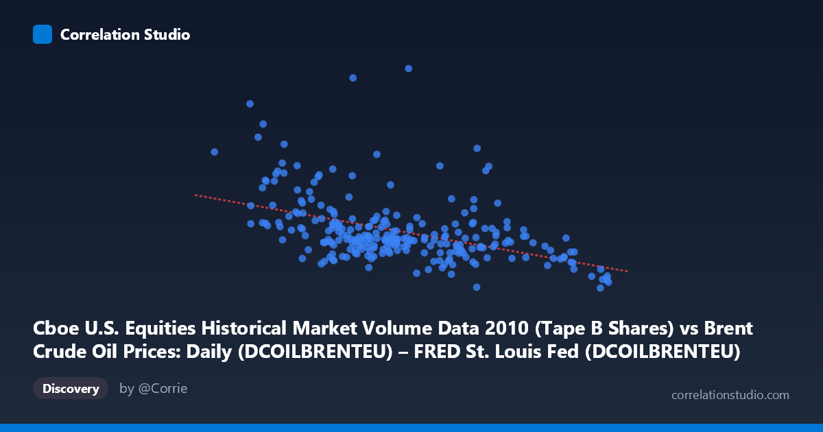
The scatterplot reveals a moderate negative relationship between Brent Crude Oil spot prices (X-axis, USD/barrel) and Cboe U.S. equity market trading volume (Y-axis, Tape B shares). The linear regression equation y = -3,484,840x + 390,336,000 indicates that for every $1 increase in crude oil price, equity trading volume decreases by approximately 3.48 million shares. Visually, while the downward trend is discernible, there is substantial scatter around the regression line, suggesting considerable unexplained variation and a relationship that is real but far from deterministic.
Correlation Strength and Statistical Significance
The correlation coefficient of r = -0.4685 indicates a moderate negative association. Crucially, the R² of 0.2195 means only ~22% of the variance in equity volume is explained by crude oil prices — leaving roughly 78% attributable to other factors. The 95% confidence interval of [-0.5597, -0.3661] is entirely negative and does not cross zero, reinforcing directional confidence, and the p-value of 3.775×10⁻¹⁵ confirms the relationship is highly statistically significant, virtually eliminating chance as an explanation given n=252. However, statistical significance with a large sample should not be conflated with practical importance — the effect size is modest. Critically, Granger causality tests find no significant predictive directionality in either direction (X→Y: F=0.85, p=0.58; Y→X: F=1.11, p=0.36), meaning that knowing past crude oil prices does not help predict future equity volumes (and vice versa) beyond baseline autoregressive patterns. This substantially weakens any causal narrative.
Notable Patterns, Clusters, and Outliers
Several features stand out in the data sample. There are notable high-volume outliers at moderate-to-low oil price levels — particularly the point at (76.48, 316,201,367) and (75.12, 195,242,236) — which exert meaningful leverage on the regression fit and suggest episodic spikes in trading activity uncorrelated with oil price levels. Conversely, the high oil price region (88–93 USD/barrel) appears clustered with consistently low volume values (45M–93M shares), which drives much of the negative correlation signal. The mid-range oil prices (74–82 USD/barrel) show the widest vertical spread in volume, indicating high heteroscedasticity — variance in trading volume is not constant across oil price levels, which violates a key assumption of simple linear regression and suggests the linear model is an oversimplification.
Confounding Factors and Caveats
Several important caveats apply. First, 2010 was a specific post-financial crisis recovery year, characterized by unusual macroeconomic dynamics including quantitative easing, sovereign debt concerns in Europe, and rebounding risk appetite — all of which independently influenced both crude prices and equity volumes. Second, equity trading volume is driven by many structural factors including earnings seasons, index rebalancing, algorithmic trading activity, and volatility regimes (VIX levels), none of which are captured here. Third, the Tape B designation covers specific exchanges (NYSE American, NYSE Arca, etc.) rather than total market volume, potentially introducing selection bias. Fourth, the axis labeling appears transposed in the original dataset description (X is labeled as volume data, Y as crude price), which warrants verification before acting on directional interpretations. Finally, the relationship observed in a single calendar year may not generalize across different market regimes.
Actionable Insights and Further Investigation
Given the moderate correlation with no confirmed Granger causality, this relationship is best interpreted as coincidental co-movement within a specific macro environment rather than a predictive or causal link. Recommended next steps include: (1) extending the analysis across multiple years (2008–2023) to test whether the negative correlation is stable or regime-dependent; (2) controlling for VIX (market volatility), S&P 500 returns, and Fed policy variables in a multivariate regression to isolate any independent crude oil effect; (3) applying a non-linear or quantile regression framework to address the evident heteroscedasticity; (4) investigating the high-volume outlier points individually, as they may correspond to identifiable market events (e.g., Flash Crash aftermath, options expiration days) that confound the baseline relationship; and (5) testing the relationship using total market volume rather than Tape B alone to assess robustness.
X dataset: Brent Crude Oil Prices: Daily (DCOILBRENTEU) – FRED St. Louis Fed
Y dataset: Cboe U.S. Equities Historical Market Volume Data 2010
Part of experiment: Daily - Brent Crude Oil Prices: Daily (DCOILBRENTEU) – FRED St. Louis Fed vs Cboe U.S. Equities Historical Market Volume Data 2010