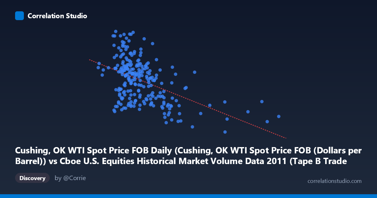
Cushing, OK WTI Spot Price FOB Daily (Cushing, OK WTI Spot Price FOB (Dollars per Barrel)) vs Cboe U.S. Equities Historical Market Volume Data 2011 (Tape B Trade Count)
- Pearson correlation (r)
- -0.4891
- Spearman correlation
- -0.4243
- p-value
- 0
- Sample size (n)
- 252
- 95% confidence interval
- -0.5777 to -0.389
- Granger causality
- None
- Granger optimal lag
- 1
AI analysis
Analysis: WTI Crude Oil Spot Price vs. Cboe Tape B Trade Count (2011)
Relationship Overview
The scatterplot reveals a moderate negative relationship between WTI crude oil spot prices (X-axis, ranging roughly from $109 to $832 per barrel equivalent in the dataset's units) and Cboe Tape B trade counts (Y-axis, ranging from approximately 75 to 113). As oil prices increase, equity trade counts on Tape B tend to decline. The linear regression equation (y = -3.77×10⁻⁵x + 105.50) confirms this inverse slope, meaning that for every unit increase in WTI price, Tape B trade count decreases by a small but consistent amount. Visually, the cloud of points slopes downward from left to right, though with considerable scatter around the trend line, suggesting the relationship is real but far from deterministic.
Correlation Strength and Statistical Significance
The Pearson correlation of r = -0.4891 indicates a moderate negative association. Critically, the R² of 0.2392 tells us that WTI spot prices explain only about 24% of the variance in Tape B trade counts — meaning roughly 76% of the variation remains unexplained by this relationship alone. While statistically highly significant (p = 2.22×10⁻¹⁶, effectively zero), this significance is partly a function of the large population size (N = 3,780), which gives enormous statistical power to detect even modest effects. The 95% confidence interval for r of [-0.578, -0.389] is reasonably tight and excludes zero, confirming the negative direction is reliable. However, the Granger causality results are notably absent in both directions — neither X→Y (F = 0.005, p = 0.945) nor Y→X (F = 3.14, p = 0.078) reaches conventional significance — meaning that neither variable temporally predicts the other in a lead-lag framework. This is a crucial caveat: the contemporaneous correlation exists, but there is no evidence that one variable drives the other forward in time.
Notable Patterns and Outliers
The scatter is heterogeneous across the X range. The bulk of observations cluster between roughly X = 150,000–400,000, where the negative trend is most visible but also where variance in Y is highest (trade counts spanning nearly the full 75–113 range). At higher X values (above ~450,000), the data becomes sparser, and trade counts appear to settle in a narrower mid-range band (roughly 85–100), which could reflect a floor effect or simply reduced sample density. Several potential outliers are visible: points like (174,908, 111.68) and (293,331, 110.60) show high trade counts at relatively low-to-moderate oil prices, while (381,544, 78.93) and (374,519, 82.32) show unusually low trade counts. These extremes may correspond to specific market events in 2011, such as the Arab Spring oil price spike in Q1 or the August debt-ceiling market turmoil, which could simultaneously depress trade counts and distort oil prices.
Confounding Factors and Caveats
Several important caveats apply. First, 2011 was an unusual year marked by the Libyan civil war, the Fukushima disaster, the U.S. debt ceiling crisis, and European sovereign debt fears — all of which affected both equity market activity and oil prices in potentially correlated but non-causal ways. A common driver (e.g., broad macroeconomic risk sentiment or market volatility regimes like the VIX) may be responsible for both moving in tandem, constituting classic confounding. Second, Tape B specifically covers NYSE American (AMEX) and regional exchange listings, which may have sector-specific exposure (e.g., energy or small-cap stocks) that creates a mechanical link to oil prices without a generalizable causal story. Third, daily autocorrelation in both time series (common in financial data) can inflate apparent correlations and reduce the effective degrees of freedom below the nominal n = 252, making statistical inferences less reliable than the p-value alone suggests. The failed Granger tests reinforce that no clean temporal mechanism has been identified.
Actionable Insights and Further Investigation
Given that the correlation exists but causality is unclear, several investigative steps would be valuable. Researchers should control for market-wide volatility (e.g., VIX) and overall market volume as covariates to determine whether the WTI–Tape B relationship survives multivariate adjustment. It would also be worthwhile to segment the year by regime (pre/post August 2011 volatility shock) to test whether the correlation is period-specific rather than structural. Extending the analysis to multiple years would clarify whether 2011 is representative or anomalous. Testing Granger causality at longer lags (beyond the optimal lag-1 tested here) could reveal slower-moving predictive relationships. Finally, examining whether energy sector stocks specifically (many of which trade on Tape B) account for the bulk of the relationship would help determine whether this is a sector-concentration artifact rather than a broad market phenomenon.
X dataset: Cboe U.S. Equities Historical Market Volume Data 2011
Y dataset: Cushing, OK WTI Spot Price FOB Daily
Part of experiment: Daily - Cboe U.S. Equities Historical Market Volume Data 2011 vs Cushing, OK WTI Spot Price FOB Daily