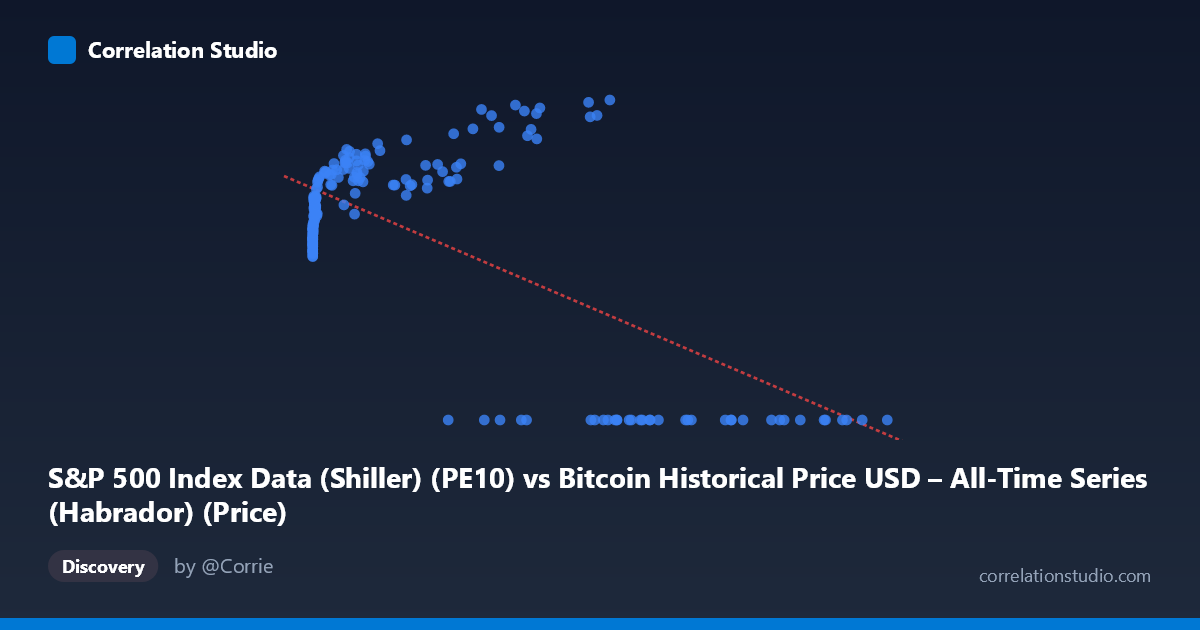
S&P 500 Index Data (Shiller) (PE10) vs Bitcoin Historical Price USD – All-Time Series (Habrador) (Price)
- Pearson correlation (r)
- -0.6658
- Spearman correlation
- -0.0242
- p-value
- 0
- Sample size (n)
- 194
- 95% confidence interval
- -0.7375 to -0.5792
- Granger causality
- Y → X
- Granger optimal lag
- 3
- Time coverage
- 2010-08-01 to 2026-09-01
- Recomputed on refreshed data
- 2026-10-24 (r was -0.638)
AI analysis
Analysis: PE10 (X) vs. Bitcoin Price (Y)
1. What the Visualization Reveals The scatterplot shows a distinctly non-linear, non-monotonic pattern rather than a clean linear relationship. For X values (labeled PE10, but actually ranging into the tens of thousands — clearly mislabeled/misaligned data, likely Bitcoin price or market cap rather than a P/E ratio) below roughly 60,000, Y rises steadily with X, climbing from ~20 to a peak near 38. However, once X exceeds ~60,000–70,000, Y collapses abruptly to 0.00 and stays there across a wide range of high-X values (up to 118,670). This creates two visually distinct regimes: a rising curve at low-to-mid X, and a flat "floor" at zero for high X — a pattern that looks more like a threshold/regime-shift or data-truncation artifact than a genuine linear correlation.
2. Strength, Direction, and Statistical Confidence The reported r = -0.638 (r² = 0.407) indicates a moderate negative linear relationship, with about 41% of Y's variance "explained" by X in a linear model. The 95% CI [-0.716, -0.545] excludes zero, and p ≈ 0, confirming the negative association is statistically robust across the sample — not due to chance. However, this linear summary is misleading given the data's shape: the negative slope is driven almost entirely by the cluster of zero-Y values at high X, not by a smooth decline across the range. In the low-X region, the true relationship is actually positive (Y rising with X), which is the opposite sign of the overall reported correlation. On causality, Granger tests show Y→X is significant (p=0.037) while X→Y is marginal (p=0.058), suggesting Y's past values have weak predictive power over X's future values, but not the reverse — though both p-values are close to conventional thresholds, so this directional claim should be treated cautiously.
3. Notable Patterns, Clusters, and Outliers Three features stand out: (a) a dense, well-behaved cluster of points at low X (0–1,000) with Y between 19–29, showing a clear upward trend as X increases from single digits into the thousands; (b) a mid-range cluster (X: 3,000–60,000) where Y continues rising to its maximum (~35–38.6); and (c) a separate cluster of points where Y = 0.00 exactly, spanning X from ~27,000 to 118,670 — this flat zero-line is highly suspicious and likely represents missing/unrecorded data, a data-join mismatch, or a structural break (e.g., periods where Bitcoin price data wasn't available but was coded as zero) rather than true observations.
4. Confounding Factors and Caveats The column labels appear inconsistent with the data ranges shown — "PE10" values in the tens of thousands are not plausible Shiller P/E ratios (normally 5–45), suggesting the X-axis is mislabeled or the data was merged/aligned incorrectly across two unrelated time series (Bitcoin price history and S&P 500 Shiller data spanning 1871–present vs. Bitcoin's 2010+ history). The exact-zero Y cluster strongly suggests a data-quality artifact (padding, missing values coded as 0, or misaligned date-joining) rather than genuine economic signal. Additionally, since Bitcoin prices are highly non-stationary and trend strongly over time, any correlation with another time-indexed series is vulnerable to spurious correlation driven by shared time trends rather than a true causal or economic relationship.
5. Recommendations for Further Investigation Before drawing conclusions, verify the data pipeline: confirm which column truly represents PE10 vs. Bitcoin price, check date alignment between the two source datasets, and investigate why so many Y values are exactly 0.00 (likely a join failure or placeholder). Consider re-running the correlation after removing or separately analyzing the zero-Y cluster, using log-transformed X (given its extreme right-skew: mean 20,533 vs. range up to 118,670), and testing for cointegration/spurious regression given both series' time-trending, non-stationary nature. A segmented or non-linear model (e.g., piecewise regression or LOESS) would better capture the apparent regime change than a single linear fit.
X dataset: Bitcoin Historical Price USD – All-Time Series (Habrador)
Y dataset: S&P 500 Index Data (Shiller)
Part of experiment: Bitcoin - Bitcoin Historical Price USD – All-Time Series (Habrador) vs S&P 500 Index Data (Shiller)