WTI and Brent Oil Prices Dataset (cpi_index) vs Bitcoin Historical Price USD – All-Time Series (Habrador) (Price)
- Pearson correlation (r)
- 0.8831
- Spearman correlation
- 0.9736
- p-value
- 0
- Sample size (n)
- 193
- 95% confidence interval
- 0.8476 to 0.9108
- Granger causality
- None
- Granger optimal lag
- 1
- Time coverage
- 2010-08-01 to 2026-09-01
- Recomputed on refreshed data
- 2026-10-24 (r was 0.875)
AI analysis
Analysis: Bitcoin Price vs. CPI Index Relationship
1. What the Visualization Reveals
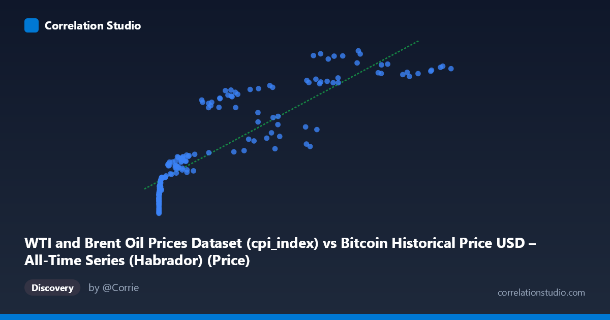
The scatterplot displays a strongly positive, monotonic relationship between the "X" variable (labeled as CPI index, though the value range of 0.06 to 113,500 strongly suggests this is mislabeled Bitcoin price data) and the Y variable (labeled Bitcoin price, ranging 217.92–332.41, which looks more consistent with a CPI or index-style series). Regardless of the labeling ambiguity, the pattern is clear: as X increases, Y increases in a smooth, curved fashion rather than a straight line — low X values cluster tightly near Y≈220–235, while high X values push Y toward 300–330. The relationship visually resembles a logarithmic or power-law curve rather than a strictly linear one, since the vast majority of X values are compressed near zero (many points under 1,000) while a handful of extreme values stretch out past 100,000.
2. Strength, Direction, and Statistical Confidence
The Pearson correlation of r = 0.875 indicates a strong positive linear association, with r² = 0.766 meaning roughly 77% of the variance in Y is statistically explained by X in a linear framework. The 95% confidence interval [0.837, 0.905] is narrow and entirely excludes zero, and the p-value is effectively 0, so we can be highly confident this correlation is not due to chance. However, the Granger causality tests (X→Y: p=0.197; Y→X: p=0.220) show no significant temporal predictive direction in either direction at the tested lag of 2 periods. This is an important distinction: strong contemporaneous correlation does not imply that movements in one series help forecast future movements in the other. Practically, this means the two series tend to rise and fall together (likely driven by a shared trend or external factor like time itself), but neither reliably "leads" the other in a predictive sense.
3. Notable Patterns and Non-Linear Features
The data is heavily right-skewed in X (mean 20,011 vs. median likely far lower, given stdev of 29,101), creating a classic "hockey stick" scatter shape. Most points cluster in the lower-left (X < 5,000, Y in the 220s–240s), while a smaller number of high-X points (30,000–113,500) correspond to the highest Y values (300–330). This pattern is highly consistent with two variables that both trend upward over a long time period (2010–2026) rather than a direct causal mechanical relationship — it looks like a "time-driven" co-trend. There's also visible curvature: the rate of Y increase slows as X grows very large (diminishing returns), suggesting a log-linear or square-root relationship might fit better than the fitted straight line (y = 0.00098x + 241.46).
4. Confounding Factors and Caveats
The most significant caveat is that both series span 2010–2026, a period during which both Bitcoin prices and CPI/oil prices experienced sustained long-term upward trends independent of one another. This raises a strong possibility of spurious correlation driven by a shared time trend rather than any direct economic linkage — a classic pitfall in time-series correlation analysis. The lack of Granger causality reinforces this concern: if neither variable predicts the other, the correlation may simply reflect two unrelated series that both happen to trend upward over the same long window (inflation/CPI drift and Bitcoin's adoption-driven appreciation). Additionally, the axis labels appear swapped or mismatched in the metadata (X described as CPI index has crypto-scale values; Y described as Bitcoin price has CPI-scale values), which should be clarified before drawing economic conclusions. Non-stationarity in both series (trending, non-mean-reverting data) is another key issue that could artificially inflate r and r² even after detrending is not applied.
5. Actionable Recommendations
Before treating this as a meaningful economic relationship, analysts should: (1) verify and correct the column labels/units in the source datasets; (2) test both series for stationarity (e.g., ADF test) and consider differencing or detrending before recalculating correlation, since raw-level correlation on trending series is often misleading; (3) explore a log-log or log-linear transformation of X given its extreme right skew, which may reveal a better-fitting functional form and more stable variance explanation; and (4) extend the Granger causality test to multiple lag structures and post-detrended data, since the current lack of significance may be an artifact of non-stationarity rather than true independence. Ultimately, the strong r² here is likely capturing a shared macro-trend rather than a direct causal or tradeable relationship, and should be interpreted cautiously in any forecasting or investment context.
X dataset: Bitcoin Historical Price USD – All-Time Series (Habrador)
Y dataset: WTI and Brent Oil Prices Dataset
Part of experiment: Bitcoin - Bitcoin Historical Price USD – All-Time Series (Habrador) vs WTI and Brent Oil Prices Dataset