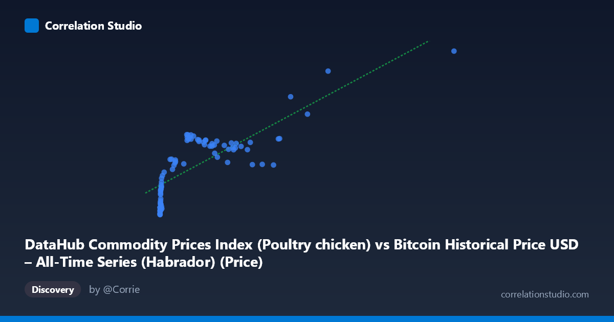
DataHub Commodity Prices Index (Poultry chicken) vs Bitcoin Historical Price USD – All-Time Series (Habrador) (Price)
- Pearson correlation (r)
- 0.7958
- Spearman correlation
- 0.7949
- p-value
- 0
- Sample size (n)
- 83
- 95% confidence interval
- 0.7003 to 0.8633
- Granger causality
- None
- Granger optimal lag
- 1
- Time coverage
- 2010-08-01 to 2017-06-01
- Recomputed on refreshed data
- 2026-10-24 (r was 0.7958)
AI analysis
Analysis: Bitcoin Price vs. Poultry Commodity Index
1. What the Visualization Reveals
The scatterplot shows a positive, generally monotonic relationship between Bitcoin's USD price (X-axis) and a poultry/chicken commodity price index (Y-axis). The data is heavily clustered at low X-values (below ~1000, representing Bitcoin's early years), with a long tail extending to the maximum of 2452.18. The relationship appears curvilinear rather than strictly linear—Y rises steeply from ~85 to ~115 as X moves from 0 to ~250, then plateaus in the 104-115 range through the middle X-range, before climbing again sharply toward 140-148 at the highest X-values (1000).
2. Strength, Direction, and Statistical Confidence
The correlation coefficient (r = 0.7958, r² = 0.633) indicates a strong positive linear association, with roughly 63% of the variance in the commodity index explained by Bitcoin price movements. The 95% CI [0.70, 0.86] is reasonably tight and excludes zero, and the p-value of ~0 confirms this correlation is highly unlikely to be due to chance in this sample. However, the Granger causality tests are critical here: neither direction shows significant predictive power (X→Y: p=0.73; Y→X: p=0.55). This means despite the strong contemporaneous correlation, Bitcoin price does not temporally predict poultry prices, nor vice versa. This strongly suggests the correlation is not causal but likely driven by a shared underlying trend (e.g., both series trending upward over 2010-2017 due to unrelated macro factors, inflation, or simple time-based drift).
3. Notable Patterns and Outliers
Three visible clusters emerge: (1) a dense cloud of low-X points (X<50) with Y ranging 85-101, representing Bitcoin's pre-2013 genesis period; (2) a mid-range cluster (X: 100-1000) where Y stabilizes around 104-116 despite substantial X variation—this plateau suggests weak local correlation within this band; (3) a sparse set of high-leverage points (X1000, particularly the 2452.18/148.38 point) that appear to disproportionately drive the overall linear fit. The relationship looks more like two or three regime segments than a single linear trend, hinting at non-linearity that the linear R²=0.633 may overstate as a "clean" relationship.
4. Confounding Factors and Caveats
The most obvious confound is time itself: both Bitcoin price and commodity indices have historically trended upward over 2010-2017 due to independent macro drivers (Bitcoin adoption/speculation cycles vs. global food/agricultural supply-demand and inflation). This is a classic case of spurious correlation via co-trending non-stationary time series. Neither series was likely detrended or differenced before correlation testing, which can artificially inflate r for any two upward-trending series. Additionally, the small effective sample (n=83) and extreme leverage from a handful of high-X outliers (Bitcoin's 2017 bull run) may be disproportionately influencing both r and the regression slope.
5. Recommendations for Further Investigation
Before drawing any economic conclusions, analysts should: (a) difference or detrend both series (e.g., use month-over-month % change) and re-test correlation—this is the standard fix for spurious time-trend correlations; (b) test for cointegration if a genuine long-run equilibrium relationship is hypothesized; (c) examine sensitivity of r² by removing the top 3-5 high-Bitcoin-price outliers; and (d) consider that the non-significant Granger results already caution against any predictive/causal framing—this relationship should be treated as coincidental co-movement rather than evidence that Bitcoin prices influence, or are influenced by, poultry commodity prices.
X dataset: Bitcoin Historical Price USD – All-Time Series (Habrador)
Y dataset: DataHub Commodity Prices Index
Part of experiment: Bitcoin - Bitcoin Historical Price USD – All-Time Series (Habrador) vs DataHub Commodity Prices Index