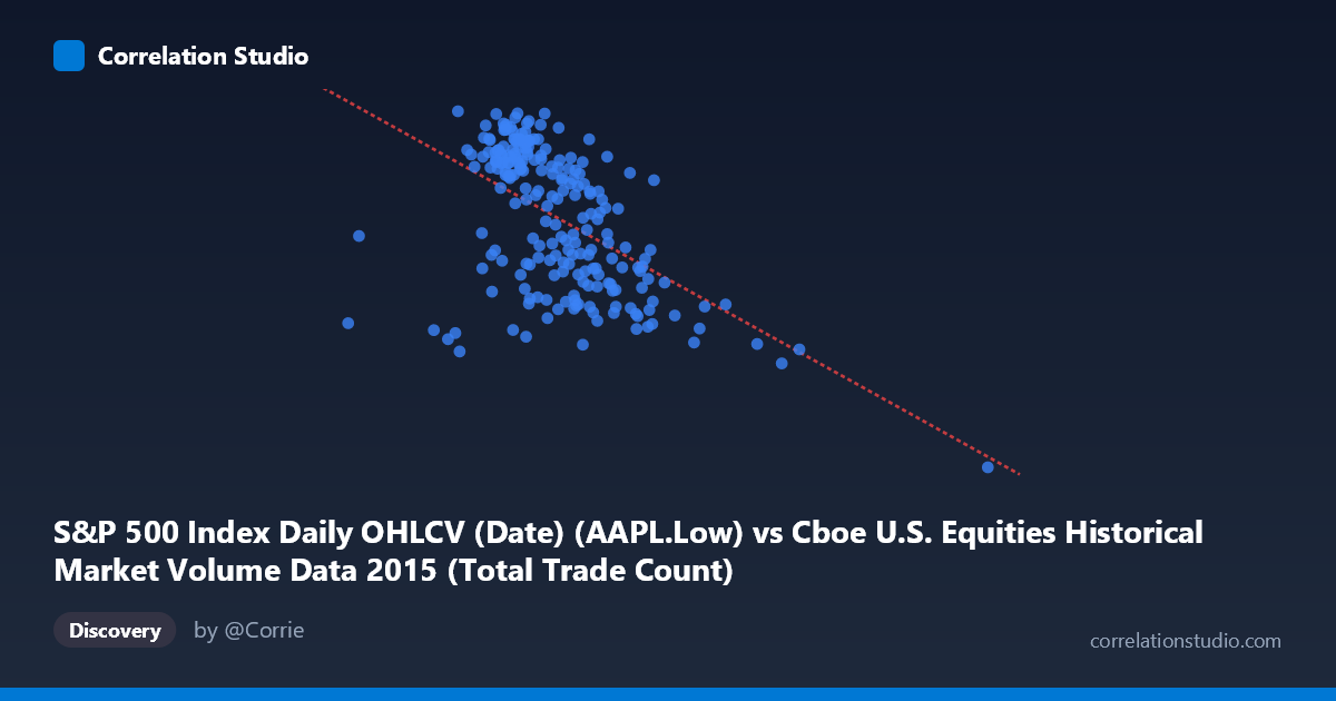
S&P 500 Index Daily OHLCV (Date) (AAPL.Low) vs Cboe U.S. Equities Historical Market Volume Data 2015 (Total Trade Count)
- Pearson correlation (r)
- -0.537
- Spearman correlation
- -0.5435
- p-value
- 0
- Sample size (n)
- 222
- 95% confidence interval
- -0.6245 to -0.4362
- Granger causality
- None
- Granger optimal lag
- 1
AI analysis
Scatterplot Analysis: AAPL Low Price vs. Cboe Total Trade Count (2015)
Relationship Overview The scatterplot reveals a moderate negative relationship between Apple's daily low price (X-axis) and the Cboe U.S. Equities total trade count (Y-axis) over the course of 2015. As AAPL's low price increases, total trade count tends to decline — suggesting that on days when Apple traded at higher price levels, overall market trade activity was somewhat lower, and vice versa. The linear regression equation (y = −8.63×10⁻⁶x + 141.07) reflects this downward slope, though the scatter around the line is considerable, indicating meaningful noise beyond the linear trend.
Correlation Strength and Statistical Significance The Pearson correlation of r = −0.537 indicates a moderate negative association, but the explained variance tells a more cautious story: R² = 0.288, meaning only about 28.8% of the variance in total trade count is accounted for by AAPL's low price. The remaining ~71% is driven by other factors entirely. The 95% confidence interval [−0.625, −0.436] is reasonably tight and does not cross zero, and the p-value is effectively zero, confirming the correlation is highly statistically significant and not a sampling artifact. However, statistical significance should not be conflated with practical importance — the modest R² limits the predictive utility of this relationship alone. Importantly, Granger causality testing found no significant directional predictive relationship in either direction (X→Y: F = 0.372, p = 0.543; Y→X: F = 0.008, p = 0.929), meaning AAPL's low price does not temporally predict trade count, nor does trade count predict AAPL's low price in a lagged sense. This strongly suggests the observed correlation is contemporaneous and likely driven by shared market forces rather than a causal mechanism.
Notable Patterns, Clusters, and Outliers The bulk of observations cluster between roughly AAPL low prices of $2.0M–$2.8M (in the encoded X units) and trade counts of 110–131, forming a relatively dense central mass with visible downward drift. Two prominent outliers stand out: one point near (5,549,284, 92.00) representing an extreme high-X, low-Y value that lies far from the main cluster and likely exerts disproportionate leverage on the regression slope. Another cluster of lower-X values (around 1.0–1.7M) also appears somewhat isolated. These extreme observations may correspond to specific high-volatility market events in 2015 (e.g., the August market correction). There is also a hint of heteroscedasticity — variance in Y appears somewhat higher at mid-range X values — and possibly a non-linear (concave) pattern, suggesting a simple linear model may not fully capture the relationship.
Confounding Factors and Interpretive Caveats Several important caveats apply. First, the axis labels appear swapped in the dataset metadata — the X-axis is labeled as drawn from the Cboe dataset but described as AAPL Low price, and vice versa, which warrants verification before drawing firm conclusions. Second, both variables are time-indexed across 2015, meaning shared macroeconomic conditions (e.g., the August 2015 Chinese market shock, Fed rate decisions, sector volatility) could simultaneously drive both AAPL prices lower and trade counts higher, producing a spurious or confounded correlation. The sample covers n = 222 paired observations from a population of N = 506 trading records, so sampling coverage is reasonable but not complete. Additionally, AAPL is a single stock, and using its low price as a proxy for broader market conditions introduces idiosyncratic stock-level noise.
Actionable Insights and Further Investigation Given the absence of Granger causality, practitioners should not use AAPL low price as a leading indicator for Cboe trade volume in any trading or risk model. However, the contemporaneous correlation does suggest that both variables respond to common latent market stress factors, making it worth investigating whether a composite market sentiment index or VIX data could better explain both. Further steps should include: (1) removing or winsorizing the extreme outlier near X = 5.55M to assess its influence on the regression; (2) testing non-linear models (e.g., polynomial or log-transformed regression) given potential curvature; (3) introducing time as an explicit variable or breaking the data into sub-periods (pre/post August correction) to detect regime changes; and (4) expanding the feature set to include volume, VIX, or sector ETF flows to build a more robust multivariate model of trade count dynamics.
X dataset: Cboe U.S. Equities Historical Market Volume Data 2015
Y dataset: S&P 500 Index Daily OHLCV (Date)
Part of experiment: Daily - Cboe U.S. Equities Historical Market Volume Data 2015 vs S&P 500 Index Daily OHLCV (Date)