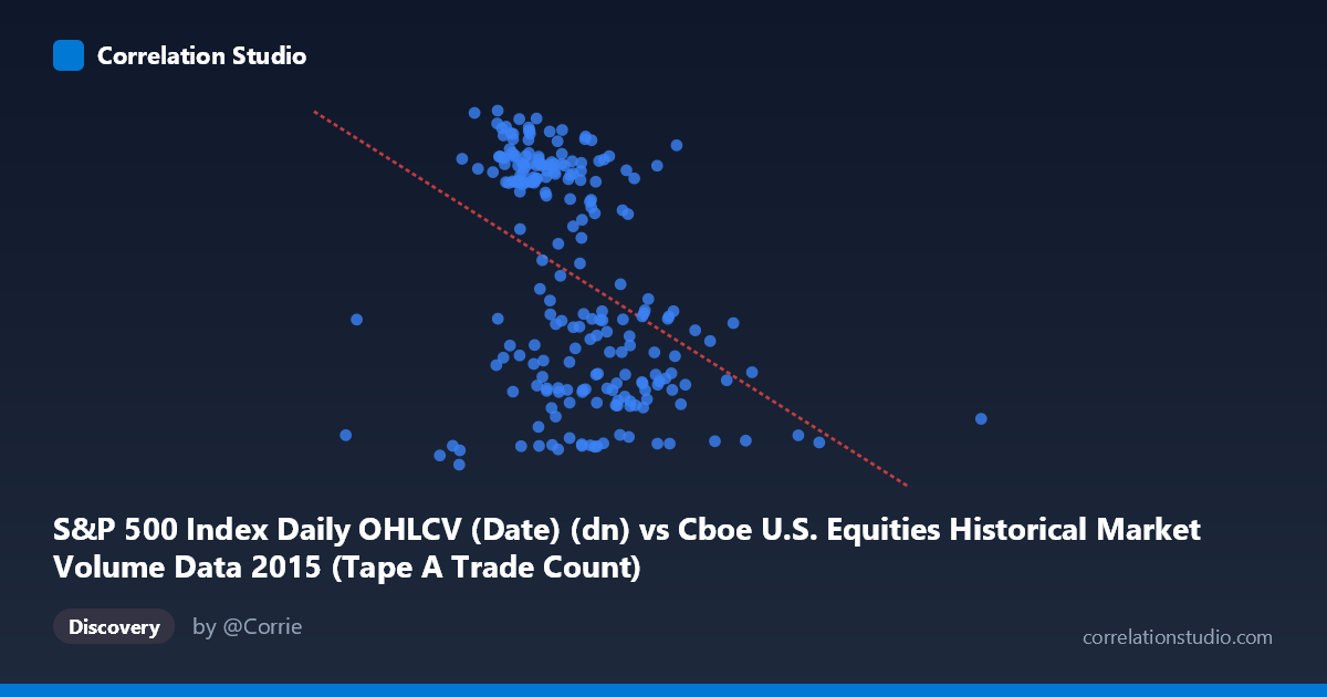
S&P 500 Index Daily OHLCV (Date) (dn) vs Cboe U.S. Equities Historical Market Volume Data 2015 (Tape A Trade Count)
- Pearson correlation (r)
- -0.4014
- Spearman correlation
- -0.445
- p-value
- 0
- Sample size (n)
- 222
- 95% confidence interval
- -0.5063 to -0.2848
- Granger causality
- None
- Granger optimal lag
- 1
AI analysis
Analysis of S&P 500 Date vs. Cboe Tape A Trade Count (2015)
Relationship Overview The scatterplot reveals a negative relationship between the S&P 500 Index date ordinal (serving as a proxy for calendar progression through 2015) and the Cboe U.S. Equities Tape A Trade Count. As the year advances from February through December 2015, Tape A trade counts show a general tendency to decline. The linear regression equation (y = -1.18×10⁻⁵x + 132.649) confirms this downward slope, suggesting that trade count activity on Tape A exchanges gradually diminished over the course of the year, though with considerable scatter around the trend line.
Correlation Strength and Statistical Significance The Pearson correlation of r = -0.4014 indicates a moderate negative association, but the explanatory power is modest: R² = 0.1611 means only ~16.1% of the variance in Tape A Trade Count is explained by the date variable. The remaining ~84% of variation is attributable to other factors entirely. The 95% confidence interval of [-0.5063, -0.2848] is entirely negative and does not cross zero, and the p-value of 5.29×10⁻¹⁰ confirms this correlation is highly statistically significant — the relationship is unlikely to be a chance finding given n = 222 paired observations. However, statistical significance should not be conflated with practical importance given the limited variance explained. Crucially, Granger causality tests reveal no significant predictive directionality in either direction (X→Y: F = 0.059, p = 0.809; Y→X: F = 0.015, p = 0.904), meaning the date does not temporally predict trade counts beyond chance, and trade counts do not predict date movement — the correlation reflects a contemporaneous trend rather than a lagged causal mechanism.
Notable Patterns, Clusters, and Outliers Several features stand out in the data. The bulk of observations cluster in the X range of approximately 1.1M to 1.6M (roughly spring through autumn 2015), where trade counts span a wide band from roughly 103 to 127 — illustrating the high day-to-day volatility in trading activity even within narrow calendar windows. There are notable outliers at very high X values: the point at (2,923,236, 105.99) and (2,247,816, 104.85) sit far to the right of the main cluster, likely representing late-year dates with suppressed trade counts, and may disproportionately influence the regression slope. At the low end of X, (616,505, 112.85) appears isolated on the left, consistent with early 2015 data. The upper Y boundary (~127) appears more frequently in mid-range X values, suggesting peak trading activity occurred in mid-year periods — potentially coinciding with volatility events such as the August 2015 market selloff.
Confounding Factors and Caveats Several important caveats apply. First, using the date column as a continuous X variable conflates calendar time with any number of market-structural, regulatory, or macroeconomic changes occurring through 2015, making it difficult to attribute the trend to any specific cause. Second, seasonality in equity market volume is well-documented (lower volume in summer, holiday periods), which may partly explain the observed decline without implying any structural shift. Third, the outlier X values (2M) are anomalous given the expected date range and may represent data entry artifacts or encoding issues that should be investigated before drawing conclusions. Fourth, the Tape A classification (NYSE-listed securities) represents only one segment of U.S. equity volume, so trends here may not generalize across Tape B or C securities. Finally, the n = 222 sample drawn from N = 506 raises questions about whether the sampling pattern (every 4th point) introduces any systematic bias.
Actionable Insights and Further Investigation Given the moderate correlation and low explained variance, practitioners should avoid using calendar date alone as a predictor of Tape A trade counts. More productive avenues include: (1) decomposing the time series using seasonal adjustment to isolate structural volume trends from cyclical patterns; (2) investigating the extreme X-value outliers to determine whether they represent legitimate late-year dates or data quality issues; (3) incorporating additional predictors such as VIX volatility, S&P 500 returns, or Federal Reserve policy events to build a more explanatory model; (4) comparing Tape A trends against Tape B and C to assess whether the decline is exchange-specific or market-wide; and (5) conducting a breakpoint or regime-change analysis around August 2015 to test whether the volume decline accelerated following the market correction, which visual inspection of the upper-Y cluster suggests may be worth pursuing.
X dataset: Cboe U.S. Equities Historical Market Volume Data 2015
Y dataset: S&P 500 Index Daily OHLCV (Date)
Part of experiment: Daily - Cboe U.S. Equities Historical Market Volume Data 2015 vs S&P 500 Index Daily OHLCV (Date)