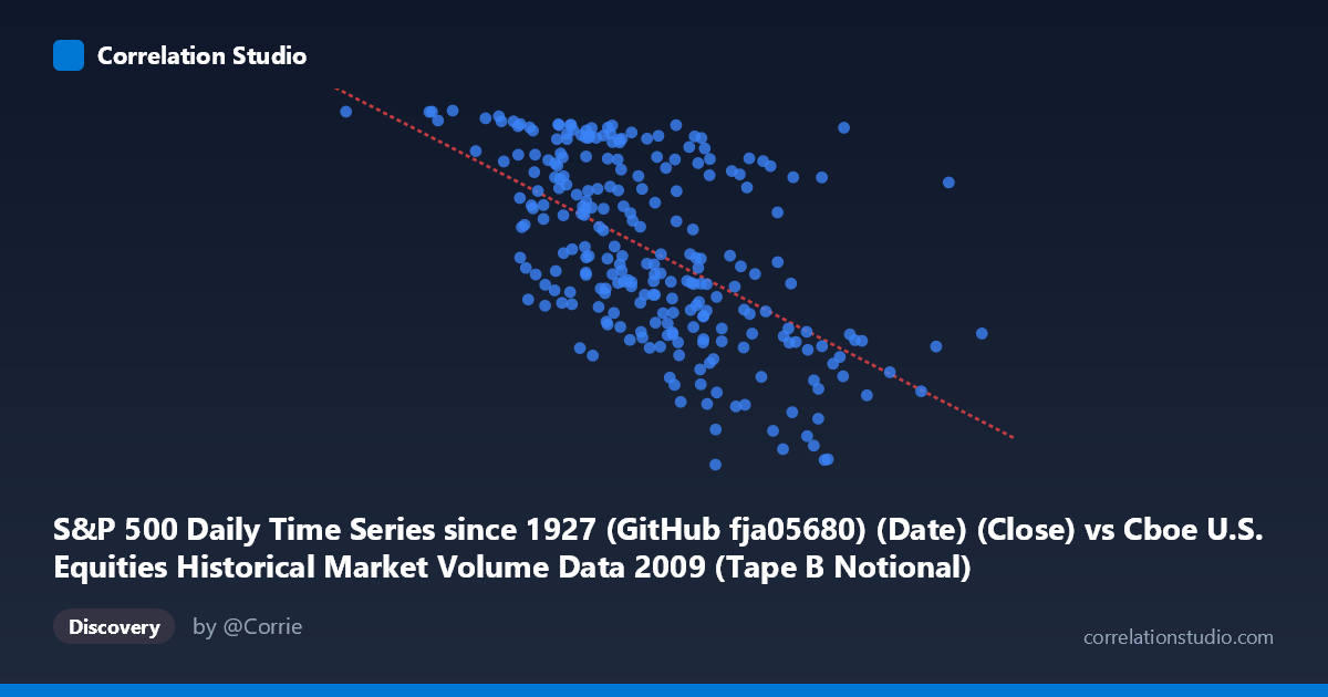
S&P 500 Daily Time Series since 1927 (GitHub fja05680) (Date) (Close) vs Cboe U.S. Equities Historical Market Volume Data 2009 (Tape B Notional)

Pearson correlation (r): -0.5785
Spearman correlation: -0.5915
p-value: 0
Sample size (n): 252
95% confidence interval: -0.6552 to -0.49
Granger causality: Bidirectional
Granger optimal lag: 10

AI analysis

Analysis: S&P 500 Close Price vs. Cboe Tape B Notional Volume (2009)

Relationship Overview The scatterplot reveals a moderate negative relationship between the S&P 500 closing price (X-axis, expressed as a date serial/timestamp value) and Cboe Tape B notional trading volume (Y-axis) across 2009. As the year progressed — with the S&P 500 recovering from its March 2009 crisis lows — Tape B notional volume generally declined. This pattern is economically intuitive: panic-driven, high-volume trading characterized the early crisis period, while the subsequent recovery was accompanied by more normalized, lower trading activity. The linear regression equation (y = -5.11×10⁻⁸x + 1217.38) captures this downward trajectory, though considerable scatter around the line is evident throughout.

Correlation Strength and Statistical Framing The Pearson correlation of r = -0.5785 indicates a moderate negative association, but the explanatory power deserves careful framing. The R² of 0.3347 means only ~33.5% of the variance in Tape B notional volume is explained by the temporal progression of S&P 500 prices — the majority (~66.5%) is attributable to other factors. The 95% confidence interval of [-0.6552, -0.4900] is meaningfully wide, reminding us that the true population correlation could range from fairly weak to moderately strong negative. The p-value of effectively zero confirms this relationship is not a statistical artifact given n=252, though statistical significance should not be conflated with practical magnitude. The bidirectional Granger causality result (X→Y: F=1.91, p=0.044; Y→X: F=1.88, p=0.049) is particularly interesting — both series appear to carry modest temporal predictive information about each other at a 10-period lag. Both F-statistics are significant but close to marginal thresholds, suggesting the predictive relationships are real but weak, and that the feedback loops between price levels and notional volume are mutually reinforcing rather than unidirectional.

Notable Patterns, Clusters, and Outliers Several structural features stand out in the sample data. A high-volume cluster is visible at lower X-values (early 2009, timestamps ~1.3B–3.9B range), where Tape B notional values reach their highest readings (~1,100–1,127), corresponding to the volatile crisis bottom period around January–March 2009. Conversely, low-volume readings congregate at higher X-values (mid-to-late 2009, ~7.0B–9.5B range), with several observations dipping below 700–750, consistent with summer/fall 2009 when markets had stabilized. There are apparent outliers at both extremes: the point near (1,320,771,983, 1126.48) and (9,511,743,751, ~low values) anchor the regression line. The relationship also appears non-linear upon close inspection — volume drops sharply through the first half of the year but plateaus or becomes more variable in the latter half, suggesting a concave or logarithmic decay rather than a strictly linear decline.

Confounding Factors and Caveats Several important caveats apply. First, X is fundamentally a time variable (encoded as Unix-style timestamps), meaning the negative correlation largely captures a time trend — both S&P 500 prices rose and Tape B volume fell over 2009 — rather than a direct price-volume causal mechanism per se. This makes standard correlation interpretation somewhat misleading. Second, Tape B specifically covers NYSE American (formerly AMEX) and regional exchange securities, which may respond differently to market conditions than the broader market captured by the S&P 500. Third, 2009 is an exceptional year — the post-crisis recovery is historically unusual, and inferences drawn here may not generalize to other periods. Fourth, the Granger causality results, while statistically significant at α=0.05, are marginal (both p-values near 0.045–0.049), and the 10-period optimal lag warrants scrutiny for economic plausibility given daily data.

Actionable Insights and Further Investigation Practitioners should consider detrending both series before computing correlation to isolate genuine price-volume dynamics from the shared time trend, using methods such as first-differencing or HP filtering. Investigating whether the relationship holds in non-crisis years would clarify whether this is a structural feature or a crisis-period artifact — a rolling correlation analysis across 1990–2024 would be valuable. Given the bidirectional Granger causality, a vector autoregression (VAR) model at 10 lags could better quantify the feedback dynamics and potentially yield short-term trading signals. Additionally, segmenting the data by market regime (bear market phase Jan–Mar vs. recovery phase Apr–Dec) could reveal whether the negative correlation is driven entirely by the early crisis period. Finally, comparing Tape B behavior against Tape A (NYSE) and Tape C (Nasdaq) in the same period would clarify whether this volume normalization pattern was exchange-specific or market-wide.

X dataset: Cboe U.S. Equities Historical Market Volume Data 2009

Y dataset: S&P 500 Daily Time Series since 1927 (GitHub fja05680) (Date)

Part of experiment: Daily - Cboe U.S. Equities Historical Market Volume Data 2009 vs S&P 500 Daily Time Series since 1927 (GitHub fja05680) (Date)