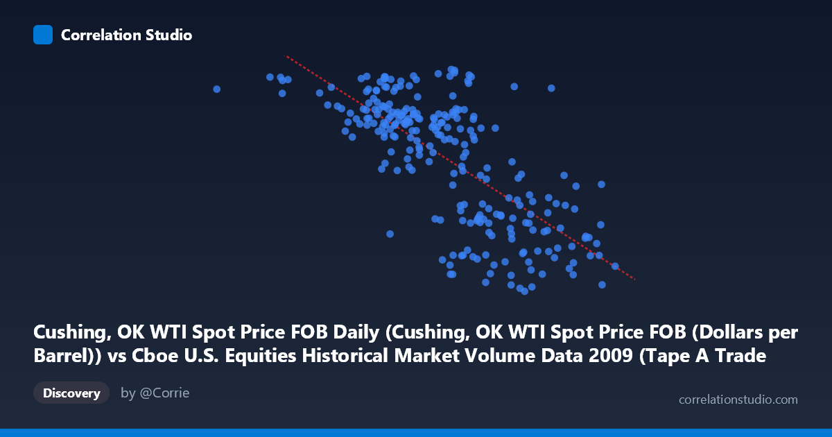
Cushing, OK WTI Spot Price FOB Daily (Cushing, OK WTI Spot Price FOB (Dollars per Barrel)) vs Cboe U.S. Equities Historical Market Volume Data 2009 (Tape A Trade Count)
- Pearson correlation (r)
- -0.7184
- Spearman correlation
- -0.7048
- p-value
- 0
- Sample size (n)
- 252
- 95% confidence interval
- -0.7733 to -0.6528
- Granger causality
- None
- Granger optimal lag
- 1
AI analysis
Analysis: WTI Crude Oil Prices vs. Cboe Tape A Trade Count (2009)
Relationship Overview The scatterplot reveals a moderately strong negative relationship between WTI crude oil spot prices (X-axis, in dollars per barrel) and Cboe Tape A trade counts (Y-axis). As oil prices rise, equity trade counts on Tape A tend to decline, and vice versa. The linear regression equation (y = -2.4714×10⁻⁵x + 102.218) captures this downward slope, with trade counts spanning roughly 34–81 units across the oil price range of ~$362 to ~$2,549 (expressed in the dataset's native units). The relationship is visually coherent — higher oil price observations cluster toward lower trade counts — though substantial scatter around the regression line indicates the relationship is real but far from deterministic.
Correlation Strength and Statistical Significance The Pearson correlation of r = -0.7184 indicates a moderately strong negative association, and the R² of 0.5161 means that approximately 51.6% of the variance in Tape A trade counts is statistically explained by WTI oil prices. This is a meaningful proportion, but it equally implies that nearly half the variance remains unexplained by this single predictor. The 95% confidence interval for r of [-0.7733, -0.6528] is relatively narrow and entirely negative, confirming consistent directional certainty. The p-value of effectively zero, combined with a sample of n = 252 drawn from a population of N = 3,232, makes the correlation highly statistically significant — this is almost certainly not a chance finding. However, Granger causality tests reveal no significant temporal predictive direction in either direction (X→Y: F = 0.59, p = 0.44; Y→X: F = 1.33, p = 0.25), meaning that neither variable reliably predicts the future values of the other at a one-period lag. This is a critical nuance: the correlation is contemporaneous, not predictive in a causal temporal sense.
Notable Patterns, Clusters, and Outliers Several structural features stand out in the data. There appear to be two loose clusters: one at lower oil prices (roughly below ~$1,200 in native units) where trade counts are predominantly elevated (60–81 range), and another at higher oil prices (above ~$1,800) where trade counts tend to compress into the 37–58 range. This bimodal clustering may reflect the dramatic oil price recovery seen during 2009 — prices collapsed in early 2009 and rebounded through the year. A few notable outliers are visible: the point at approximately (362,081, 76.83) sits at the extreme low end of oil prices with high trade count, likely representing the distressed early-2009 market environment; conversely, points near (2,549,192, 39.35) represent the high-price, low-trade-count extreme. Some high-oil-price observations also show unexpectedly elevated trade counts, suggesting the relationship is not perfectly monotonic throughout the year.
Confounding Factors and Interpretive Caveats This correlation almost certainly reflects shared temporal dynamics rather than a direct causal mechanism between oil prices and equity trade counts. Both variables were strongly influenced by the 2008–2009 financial crisis and recovery cycle: early 2009 saw depressed oil prices coinciding with peak market volatility and elevated trading volumes (fear-driven activity), while as the year progressed, oil prices recovered and equity market volatility — and with it, trade counts — normalized downward. This is a classic spurious correlation through a common confounder: macroeconomic recovery trajectory and the VIX (market volatility index) likely drive both series simultaneously. Additionally, the Granger causality failure strongly suggests the variables are co-driven by external forces rather than influencing each other. The dataset's unit encoding for oil prices (appearing in the hundreds of thousands) should also be verified for scaling consistency.
Actionable Insights and Further Investigation Given the Granger causality null result, practitioners should avoid using oil prices as a leading indicator of Tape A trade volume in short-term trading models — the predictive value at a one-period lag is statistically negligible. To properly decompose this relationship, the analysis should introduce a volatility index (VIX) or macro indicators as covariates to test whether the oil-trade-count correlation survives multivariate controls. Extending the Granger analysis to longer lags (2–10 periods) may reveal delayed transmission effects not captured at lag 1. Additionally, segmenting the data by quarter would clarify whether the correlation is stable year-round or concentrated in the high-volatility early-2009 period. Finally, examining whether similar patterns hold across other years would determine if this is a durable structural relationship or a 2009-specific artifact of extraordinary market conditions.
X dataset: Cboe U.S. Equities Historical Market Volume Data 2009
Y dataset: Cushing, OK WTI Spot Price FOB Daily
Part of experiment: Daily - Cboe U.S. Equities Historical Market Volume Data 2009 vs Cushing, OK WTI Spot Price FOB Daily