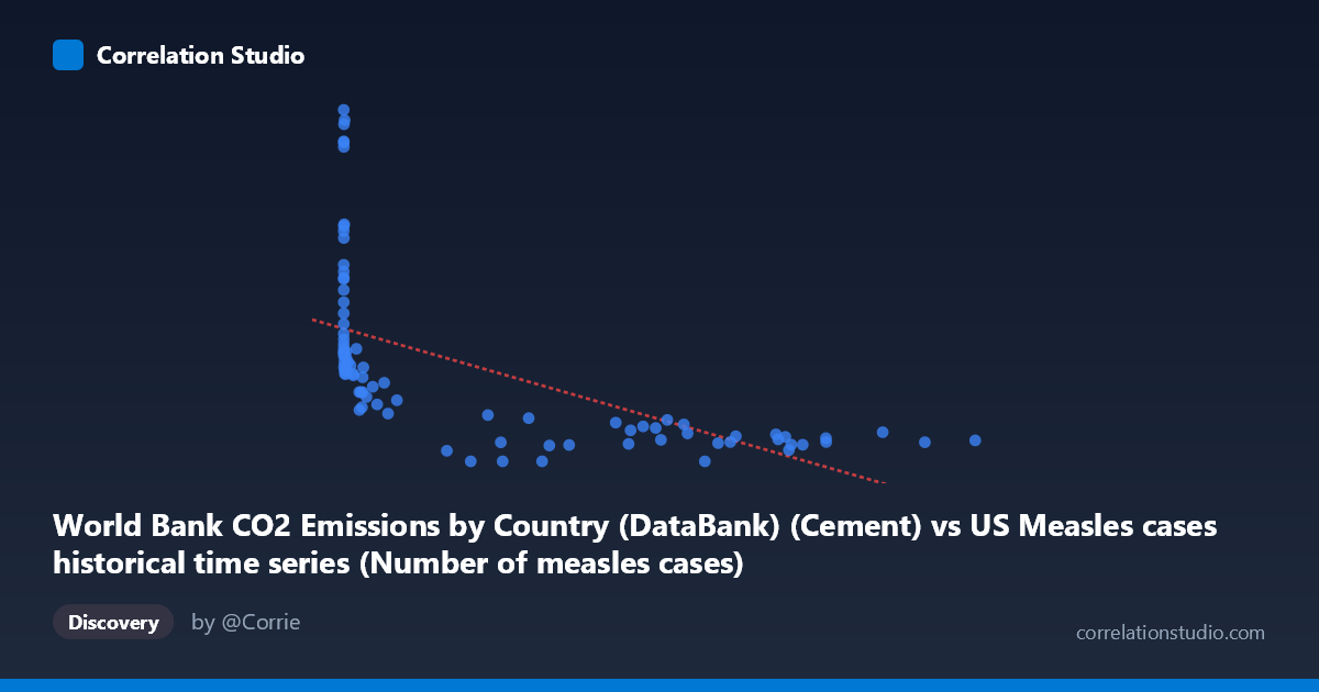
World Bank CO2 Emissions by Country (DataBank) (Cement) vs US Measles cases historical time series (Number of measles cases)
- Pearson correlation (r)
- -0.5975
- Spearman correlation
- -0.8943
- p-value
- 0
- Sample size (n)
- 87
- 95% confidence interval
- -0.7178 to -0.4425
- Granger causality
- None
- Granger optimal lag
- 10
AI analysis
Analysis: US Measles Cases vs. Global Cement CO₂ Emissions (1919–2020)
1. What the Visualization Reveals
The scatterplot displays a negative relationship between global cement-sector CO₂ emissions (X-axis) and US measles case counts (Y-axis) across roughly a century of annual observations. The most visually striking feature is a pronounced L-shaped or hyperbolic distribution: high measles case counts (700–2,600+) cluster at very low cement emission values (roughly below 50,000 units), while high emission values are associated almost exclusively with low measles counts (below ~600). This pattern immediately suggests the relationship is not truly linear but rather reflects two phenomena that both changed dramatically and monotonically over the 20th century — industrial growth and vaccine-driven disease elimination — without any direct mechanistic connection between them.
2. Correlation Strength, Direction, and Temporal Predictability
The Pearson correlation of r = −0.5975 (95% CI: [−0.7178, −0.4425], p = 1.003×10⁻⁹) is statistically highly significant, yet the R² of 0.357 means that only 35.7% of the variance in measles cases is linearly explained by cement emissions — leaving nearly two-thirds of the variance unaccounted for by this model alone. The confidence interval is relatively broad, spanning from a moderate to a strong negative correlation, reflecting real uncertainty in the precise magnitude of the relationship. Critically, the Granger causality analysis finds no significant predictive direction in either direction (X→Y: F=1.45, p=0.184; Y→X: F=0.77, p=0.656), meaning that past cement emission values do not help forecast future measles cases, and vice versa. This is a foundational result: even the statistically significant correlation carries zero temporal predictive utility, reinforcing that the association is spurious rather than causal.
3. Notable Patterns, Clusters, and Outliers
Several structural features stand out. A dense cluster of high-measles, low-emission points appears in the lower-left of the plot, corresponding to the pre-WWII era when both industrial output was lower and measles vaccination did not exist. Conversely, a horizontal band of low measles counts (0–400) stretches across the high-emission range (300,000–894,000), reflecting the post-1963 vaccine era. There are notable outliers with very high measles counts at low X values — points like (13, 2608.93), (86, 2374.89), (120, 2367.58), (1274, 2532.94), and (381, 2501.79) — likely representing epidemic years in the 1920s–1950s. Additionally, three zero-measles observations appear at mid-to-high X values, possibly reflecting reporting gaps or near-elimination years. The Spearman ρ exceeding Pearson r confirms the relationship is better described by a logarithmic or power-law curve than a straight line, consistent with the visible hyperbolic shape.
4. Confounding Factors and Caveats
This correlation is a textbook illustration of shared temporal trend confounding — both variables are strongly time-dependent and happened to move in opposite directions across the 20th century for entirely independent reasons. Cement CO₂ emissions rose due to global industrialization and population growth; measles cases fell due to the introduction of the measles vaccine in 1963, improved public health infrastructure, and mandatory school immunization programs. Time itself is the dominant hidden variable. Additional caveats include: (1) the X variable is global cement emissions while Y is US-only disease burden, making any direct linkage implausible on its face; (2) measles reporting quality changed substantially across the century; (3) the dataset labels appear transposed in the metadata (the CO₂ dataset is labeled as a measles dataset source and vice versa), warranting verification of data provenance; and (4) with n=87 over 101 years, some years may be missing or averaged, affecting temporal structure.
5. Actionable Insights and Further Investigation
The most important actionable insight is to not interpret this correlation as meaningful for policy or scientific inference — it is a spurious time-series correlation and should be treated as a methodological case study rather than a finding. For further investigation, researchers should: (1) detrend both time series (e.g., first-differencing or fitting and removing a time trend) before computing correlations, which would likely reduce r substantially toward zero; (2) fit a logarithmic regression (y = a·ln(x) + b) given the Spearman Pearson signal and visible hyperbolic shape, which would improve model fit over the linear specification; (3) examine whether interrupted time-series analysis centered on 1963 (vaccine introduction) reveals a structural break that explains the distributional shift; and (4) if the goal is genuinely to study measles determinants, substitute X with vaccination coverage rates, public health spending, or population density — variables with plausible mechanistic pathways to measles transmission.
X dataset: US Measles cases historical time series
Y dataset: World Bank CO2 Emissions by Country (DataBank)
Part of experiment: Yearly - US Measles cases historical time series vs World Bank CO2 Emissions by Country (DataBank)