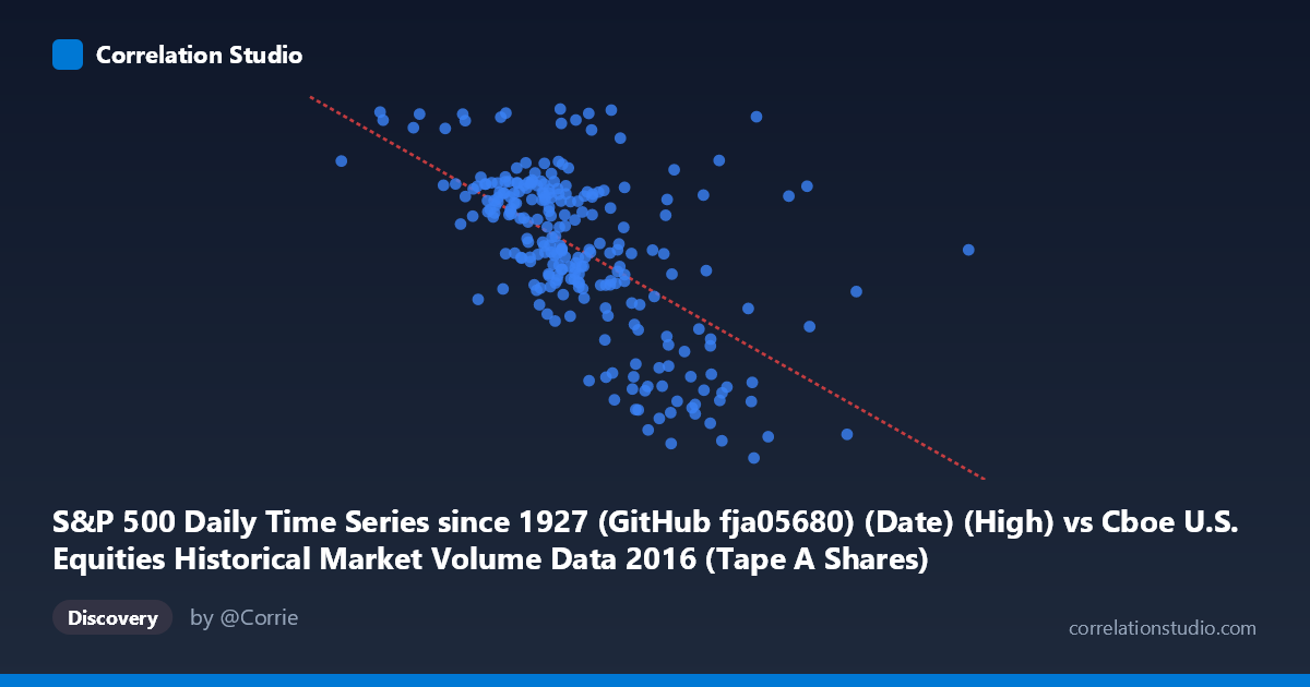
S&P 500 Daily Time Series since 1927 (GitHub fja05680) (Date) (High) vs Cboe U.S. Equities Historical Market Volume Data 2016 (Tape A Shares)
- Pearson correlation (r)
- -0.6005
- Spearman correlation
- -0.5982
- p-value
- 0
- Sample size (n)
- 252
- 95% confidence interval
- -0.6741 to -0.5152
- Granger causality
- None
- Granger optimal lag
- 4
AI analysis
Scatterplot Analysis: S&P 500 High vs. Cboe Tape A Share Volume (2016)
Relationship Overview The scatterplot reveals a moderate negative relationship between the S&P 500 daily high price and Cboe Tape A share volume throughout 2016. As the S&P 500 index reached higher price levels (roughly $105M–$543M range on the x-axis), Tape A share volume tended to decline. This inverse pattern is consistent with a well-documented market microstructure phenomenon: as equity prices rise in a trending bull market, trading activity and urgency among participants often diminish, reflecting reduced anxiety and lower turnover. The regression line (y = -1.00321E-06x + 2376.68) confirms a shallow but consistent downward slope across the observed range.
Correlation Strength and Statistical Significance The Pearson correlation of r = -0.6005 indicates a moderate negative association, with the direction being clear and consistent. However, r² = 0.3606 is the more informative metric here — it tells us that only ~36% of the variance in Tape A share volume is explained by the S&P 500 high price level. This means nearly two-thirds of the variation in trading volume is driven by factors outside this relationship. The 95% confidence interval of [-0.6741, -0.5152] is relatively tight and does not cross zero, and the p-value of effectively 0 confirms this correlation is highly statistically significant and not a sampling artifact, especially given n = 252 paired observations drawn from a population of N = 3,622. Critically, however, the Granger causality tests show no significant predictive directionality in either direction (X→Y: F = 0.503, p = 0.734; Y→X: F = 1.241, p = 0.294). This means that while the two variables are correlated contemporaneously, neither variable reliably predicts future values of the other at the tested lag structure, cautioning strongly against any causal narrative.
Notable Patterns, Clusters, and Outliers Several structural features stand out in the data. The bulk of observations cluster in the S&P 500 high range of approximately 210M–310M, where volume spans a wide band (roughly 1,900–2,250), suggesting high dispersion and heteroscedasticity in this central zone. At higher price values (330M), the data thins considerably, and volume consistently falls below ~2,100 — this upper-right sparsity likely corresponds to the late 2016 post-election rally, where prices surged but volume behavior shifted. A few notable outliers appear at lower price levels (<200M) with very high volume readings approaching 2,270+, which may correspond to high-volatility episodes in early 2016 (e.g., the January–February selloff), when fear-driven trading spiked. One point near (278M, 2272) stands out as a high-volume anomaly even at a mid-range price, possibly representing an event-driven trading surge.
Confounding Factors and Caveats Several important caveats apply. First, 2016 was an atypical year with significant macro events — the Brexit vote (June), U.S. presidential election (November), and Federal Reserve rate decisions — each of which could independently drive both price levels and volume in ways that create spurious correlation. Second, the x-axis label referencing "High" values (rather than close prices) introduces a measurement nuance: daily highs capture intraday extremes and may not best represent the prevailing price environment driving volume decisions. Third, Tape A shares specifically (NYSE-listed securities) represent only a subset of total market activity; routing and fragmentation across venues could affect this metric independently of broad market price levels. Finally, the absence of Granger causality at the 4-period optimal lag does not rule out longer-horizon predictive relationships or non-linear dependencies not captured by standard linear Granger tests.
Actionable Insights and Further Investigation Practitioners should avoid using S&P 500 price levels alone as a volume predictor given the weak explanatory power and absent Granger causality. For deeper analysis, it would be valuable to: (1) incorporate VIX (volatility index) as a likely confounding variable that independently drives both price momentum and volume; (2) test for non-linear or threshold effects, as the relationship may behave differently in high-volatility regimes versus calm trending markets; (3) segment the data by market event windows (pre/post-election, Brexit period) to assess whether the correlation is regime-dependent rather than structural; and (4) extend the Granger causality testing to longer lag structures (beyond 4 periods) and consider vector autoregression (VAR) models for a more comprehensive temporal dependency assessment. The moderate correlation is analytically interesting, but the causal ambiguity means it should inform rather than drive trading or market structure decisions.
X dataset: Cboe U.S. Equities Historical Market Volume Data 2016
Y dataset: S&P 500 Daily Time Series since 1927 (GitHub fja05680) (Date)
Part of experiment: Daily - Cboe U.S. Equities Historical Market Volume Data 2016 vs S&P 500 Daily Time Series since 1927 (GitHub fja05680) (Date)