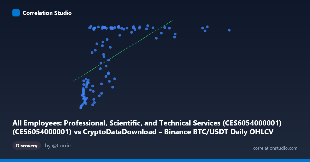
All Employees: Professional, Scientific, and Technical Services (CES6054000001) (CES6054000001) vs CryptoDataDownload – Binance BTC/USDT Daily OHLCV (tradecount)
- Pearson correlation (r)
- 0.6037
- Spearman correlation
- 0.7227
- p-value
- 0
- Sample size (n)
- 106
- 95% confidence interval
- 0.4666 to 0.7124
- Granger causality
- None
- Granger optimal lag
- 10
AI analysis
Analysis: BTC/USDT Trading Volume Proxy vs. Professional Services Employment
1. What the Visualization Reveals
The scatterplot shows a moderate positive relationship between a Binance BTC/USDT market metric (X-axis, ranging from 4,000 to over 9.39 million) and professional services employment tradecount (Y-axis, 9,094–10,821). Rather than a clean linear trend, the pattern strongly resembles a saturation or logarithmic curve: at low X values (roughly 4,000–500,000), Y climbs steeply from ~9,100 to ~10,000+, but once X exceeds ~1,000,000, Y plateaus in a tight band around 10,700–10,820 regardless of how large X grows (even out to 9.3 million). This threshold-like behavior is the dominant visual feature.
2. Strength, Direction, and Statistical Confidence
The Pearson correlation (r = 0.598, r² = 0.358) indicates a moderate positive linear association, but only explains 35.8% of the variance in Y — meaning nearly two-thirds of Y's variability is unaccounted for by a linear fit with X. The 95% CI [0.460, 0.709] is reasonably tight and excludes zero, and the p-value (1.56e-11) confirms this relationship is highly unlikely to be due to chance. However, the note that Spearman ρ exceeds Pearson r is a key signal: the rank-based correlation is stronger than the linear one, reinforcing that a logarithmic or saturating curve fits better than a straight line — consistent with the visual plateau. Critically, Granger causality tests show no significant predictive direction either way (X→Y: p=0.395; Y→X: p=0.647), meaning neither series reliably forecasts the other's future values at any of the tested lags. This strongly suggests the correlation is not causal in a temporal sense but may instead reflect a shared underlying driver, a spurious relationship from unrelated trends, or coincidental co-movement over the sample window.
3. Notable Patterns and Outliers
The clearest structural feature is the compression/saturation at high X: dozens of points with X 1M cluster tightly at Y ≈ 10,750–10,820, producing an almost flat ceiling. Conversely, the low-X region shows much more scatter and steeper sensitivity — small changes in X correspond to large swings in Y (e.g., X=4,000→Y=9,094 vs. X=638,484→Y=10,821, a huge jump over a relatively small X range). There are also several notable low-Y outliers at moderate-to-high X, such as (2,023,802 / 9,534.9), (2,147,223 / 9,710.4), and (1,314,910 / 9,603.8), which break from the plateau and pull down the linear fit's explanatory power. These look like transient dips inconsistent with the rest of the high-X cluster.
4. Confounding Factors and Caveats
This pairing is conceptually unusual: X is a daily cryptocurrency trading metric (BTC/USDT on Binance) while Y is a monthly seasonally-adjusted labor market series (professional/technical services employment). These operate on different time granularities, economic domains, and drivers — crypto trading volume responds to market speculation, volatility, and exchange-specific dynamics, while employment reflects macroeconomic labor trends, hiring cycles, and broad economic growth. Any correlation is plausibly driven by a mutual trend over time (e.g., both series rising over 2017–2026 due to unrelated secular growth — crypto adoption expanding alongside a growing economy) rather than genuine interaction. The mismatched time coverage and frequency (daily vs. monthly, resampled to n=105 pairs from N=437) also raises concerns about aggregation artifacts and lost information from downsampling.
5. Suggested Next Steps
Given the lack of Granger causality and the domain mismatch, this correlation should be treated as likely spurious or trend-driven rather than economically meaningful. To investigate further: (1) detrend both series (e.g., first-differencing or removing time trend) and re-test correlation to see if it disappears — a classic check for spurious trend correlation; (2) fit and compare a logarithmic/log-log or piecewise model given the Spearman/Pearson divergence and visible saturation; (3) align time frequencies properly (aggregate BTC data to monthly) rather than relying on arbitrary paired sampling; and (4) if a genuine relationship is suspected, search for a plausible confounding macro variable (e.g., overall market risk appetite, interest rates, or calendar time itself) that could jointly drive both series.
X dataset: CryptoDataDownload – Binance BTC/USDT Daily OHLCV
Y dataset: All Employees: Professional, Scientific, and Technical Services (CES6054000001)
Part of experiment: Bitcoin - CryptoDataDownload – Binance BTC/USDT Daily OHLCV vs All Employees: Professional, Scientific, and Technical Services (CES6054000001)