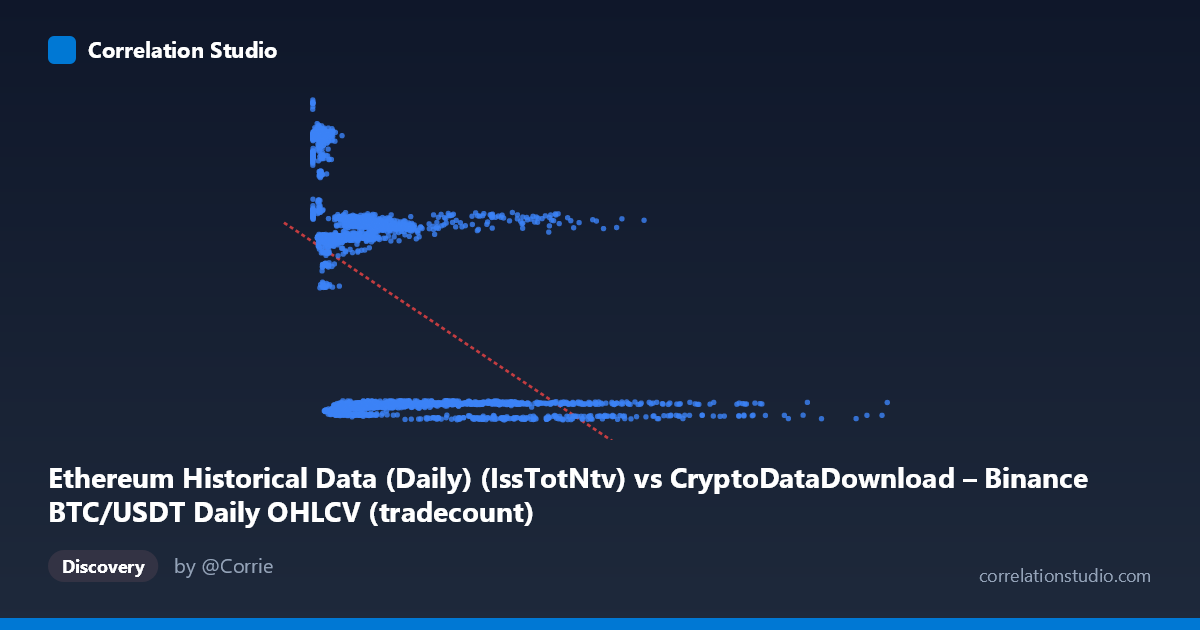
Ethereum Historical Data (Daily) (IssTotNtv) vs CryptoDataDownload – Binance BTC/USDT Daily OHLCV (tradecount)
- Pearson correlation (r)
- -0.5339
- Spearman correlation
- -0.5516
- p-value
- 0
- Sample size (n)
- 3191
- 95% confidence interval
- -0.5583 to -0.5087
- Granger causality
- None
- Granger optimal lag
- 10
- Time coverage
- 2017-08-17 to 2026-05-20
AI analysis
Analysis of the Scatterplot Relationship
1. Overview of the Relationship
The scatterplot depicts a moderate negative relationship between the X variable (labeled here as "IssTotNtv," though the column naming/dataset labeling appears mismatched with actual BTC/ETH descriptions) and Y ("tradecount"). Visually, the data does not form a tight linear band but instead shows a fan-shaped or clustered pattern, with low-X values spreading across the full range of Y, and high-X values compressing tightly toward low Y. This suggests the relationship is not uniform across the range of X — it behaves more like a curved or threshold-based decay than a constant linear slope.
2. Strength, Direction, and Statistical Confidence
The correlation coefficient (r = -0.5339) indicates a moderate negative linear relationship: as X increases, Y tends to decrease. However, r² = 0.2851 shows that only about 28.5% of the variance in Y is explained by X — meaning over 70% of Y's variability is driven by other factors, noise, or nonlinear dynamics not captured by this simple linear model. The 95% confidence interval [-0.5583, -0.5087] is narrow, and the p-value of ~0 confirms the correlation is highly statistically significant and not due to chance — but statistical significance here reflects the large sample size (n=3,191) rather than strong predictive power. Critically, the Granger causality tests show no significant predictive direction in either direction (X→Y: p=0.17; Y→X: p=0.24) at the optimal lag of 10 periods. This means that despite the contemporaneous correlation, neither variable's past values reliably help forecast the other's future values — the relationship, whatever its cause, is not one of temporal lead-lag dynamics.
3. Patterns, Clusters, and Outliers
The sample points reveal distinct clustering rather than a smooth continuum. There appear to be at least two or three regimes in Y: a low band (~1,600–3,000), a middle band (~13,000–15,000), and a high band (~18,000–21,000). Low-X values (near zero to ~500,000) populate all three Y bands, while X values above ~2 million almost exclusively align with the low-Y band (~1,600–2,900). This clustering suggests the true relationship may be regime-dependent or driven by a categorical/temporal factor (e.g., different market periods or phases) rather than a continuous functional relationship. A few extreme X outliers (e.g., X ≈ 15.36M, or the sample point at 9,324,662) also pull heavily on the linear fit despite representing rare conditions.
4. Confounding Factors and Caveats
Several caveats are important: - Dataset mismatch: The column descriptions (BTC OHLCV "IssTotNtv" vs. Ethereum "tradecount") don't clearly correspond to the stated axis labels, raising concern about how these series were joined/aligned — verify that timestamps are correctly matched. - Time-series autocorrelation: Both variables likely trend over time (e.g., across the 2017–2026 window), so the correlation may partly reflect shared secular trends (e.g., overall crypto market growth/decline) rather than a direct causal link — a classic confounding issue in time series correlation. - Nonlinearity: The clustering pattern suggests a linear model is a poor fit; the true relationship may be exponential, logarithmic, or regime-switching. - No causal direction: The Granger test results caution strongly against interpreting this as a predictive/causal relationship in either direction.
5. Recommendations for Further Investigation
- Segment the data by time period or market regime (e.g., bull/bear cycles) to check if the negative correlation is driven by a few structural breaks rather than a continuous relationship. - Apply log transformation to X (given its huge range and right-skew: mean 1.97M vs stdev 2.24M) to test for a log-linear relationship, which may substantially improve fit. - Test for confounding trends by detrending both series (e.g., differencing or removing time-based drift) before re-assessing correlation, to isolate any relationship independent of shared temporal trends. - Investigate clustering with a regime-switching or mixture model, since the banded Y-distribution suggests discrete states rather than continuous covariation. - Given the lack of Granger causality, avoid using either variable to forecast the other; instead, treat the correlation as descriptive/contemporaneous only, and look for a third common driver (e.g., overall market cap, volume, or macro crypto sentiment) that might explain both series simultaneously.
X dataset: CryptoDataDownload – Binance BTC/USDT Daily OHLCV
Y dataset: Ethereum Historical Data (Daily)
Part of experiment: Bitcoin - CryptoDataDownload – Binance BTC/USDT Daily OHLCV vs Ethereum Historical Data (Daily)