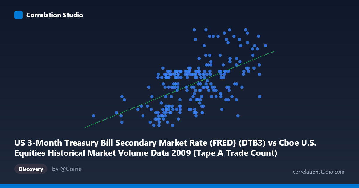
US 3-Month Treasury Bill Secondary Market Rate (FRED) (DTB3) vs Cboe U.S. Equities Historical Market Volume Data 2009 (Tape A Trade Count)
- Pearson correlation (r)
- 0.5505
- Spearman correlation
- 0.5421
- p-value
- 0
- Sample size (n)
- 250
- 95% confidence interval
- 0.4577 to 0.6315
- Granger causality
- None
- Granger optimal lag
- 1
AI analysis
Scatterplot Analysis: US 3-Month T-Bill Rate vs. Cboe Tape A Trade Count (2009)
Relationship Overview
The scatterplot reveals a moderate positive relationship between the US 3-Month Treasury Bill Secondary Market Rate and Cboe U.S. Equities Tape A Trade Count during 2009. As the T-bill rate increases, trade count tends to rise as well, with the linear regression equation y = 9.95×10⁻⁸x − 0.0120 capturing this upward trend. This is a somewhat counterintuitive pairing at first glance — one might expect higher risk-free rates to dampen equity trading activity — but 2009 was an extraordinary year marked by the post-financial-crisis recovery, making the temporal coincidence of these two variables particularly meaningful to interrogate carefully.
Correlation Strength and Statistical Significance
The Pearson correlation of r = 0.5505 indicates a moderate positive association, and the r² of 0.3031 tells us that approximately 30.3% of the variance in Tape A trade count is statistically explained by the T-bill rate level. While this is a non-trivial share, it also means nearly 70% of the variance remains unexplained by this single predictor, underscoring the limits of this relationship in isolation. The 95% confidence interval of [0.4577, 0.6315] is relatively tight given the sample size of n = 250 drawn from N = 3,232 observations, and the p-value of essentially zero confirms the correlation is highly unlikely to be a chance artifact. However, the Granger causality results are notably absent of significance in either direction — X→Y yields F = 1.85 (p = 0.175) and Y→X yields F = 0.26 (p = 0.612) — meaning neither variable temporally predicts the other at a one-period lag. This is a critical caveat: the correlation is real statistically, but there is no evidence of a predictive or causal temporal pathway between these two series.
Patterns, Clusters, and Outliers
Several structural features stand out in the sample points. There is a visible clustering of observations in the X range of roughly 1.2M–1.9M (trade count), where the T-bill rate spans broadly from ~0.03 to ~0.21, suggesting high variability in rates even at moderate trading volumes. A few points warrant attention as potential outliers: the observation at (362,081 trades, 0.05 rate) sits far to the left of the distribution and likely corresponds to an early-January low-volume session, while (2,549,191 trades, 0.27 rate) and (2,473,941 trades, 0.18 rate) anchor the upper-right region. Additionally, there are cases of similar trade volumes paired with very different rates (e.g., ~1.66M trades at both 0.06 and 0.29), suggesting heteroscedasticity — variance in Y appears to increase with X, which could violate linear regression assumptions and slightly inflate confidence in the fit.
Confounding Factors and Caveats
The most significant interpretive caveat here is shared temporal trend (spurious correlation). In 2009, both equity trading volumes and short-term interest rates followed macro-driven trajectories tied to the Federal Reserve's emergency monetary policy response and the equity market's post-crisis volatility and recovery. The Fed cut rates to near-zero by year-end, while trading volumes spiked during high-volatility periods early in the year and again during the spring rally. Both variables are therefore likely jointly driven by a third factor — market stress and macroeconomic uncertainty — rather than causally linked to each other. Additionally, the dataset covers only a single calendar year, limiting generalizability and making any trend-driven correlation susceptible to being a spurious artifact of shared time-series drift. The axis labels also appear inverted in the dataset metadata (X/Y dataset descriptions are swapped), which warrants verification before drawing firm conclusions.
Actionable Insights and Further Investigation
Given the significant correlation but absent Granger causality, the most productive next steps would be to: (1) detrend both series (e.g., first-differencing or removing seasonal components) to test whether the correlation persists after removing shared macro trends; (2) introduce control variables such as the VIX volatility index, S&P 500 return, or Fed policy event dummies, which are plausible common drivers; (3) extend the time window beyond 2009 to test whether this r ≈ 0.55 relationship holds across different rate regimes (e.g., 2015–2018 rate hike cycle vs. 2020 zero-rate environment); and (4) test non-linear specifications, since the heteroscedasticity visible in the scatter suggests a log-transformed or polynomial model may better characterize this relationship. The 2009 single-year framing is analytically limiting, and this correlation is best treated as a hypothesis-generating finding rather than a robust structural relationship.
X dataset: Cboe U.S. Equities Historical Market Volume Data 2009
Y dataset: US 3-Month Treasury Bill Secondary Market Rate (FRED)
Part of experiment: Daily - Cboe U.S. Equities Historical Market Volume Data 2009 vs US 3-Month Treasury Bill Secondary Market Rate (FRED)