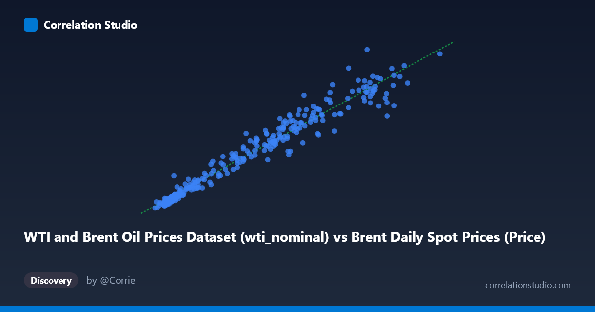
WTI and Brent Oil Prices Dataset (wti_nominal) vs Brent Daily Spot Prices (Price)
- Pearson correlation (r)
- 0.9777
- Spearman correlation
- 0.9813
- p-value
- 0
- Sample size (n)
- 295
- 95% confidence interval
- 0.972 to 0.9822
- Granger causality
- None
- Granger optimal lag
- 2
AI analysis
Analysis: WTI Nominal vs. Brent Real (CPI-Adjusted) Oil Prices
1. Overall Relationship The scatterplot reveals a strikingly tight, positive linear relationship between Europe Brent nominal spot prices and CPI-adjusted WTI crude prices. Points cluster closely along a well-defined diagonal, confirming that these two benchmarks move in near-lockstep across the full 1987–2026 time horizon. The regression equation (y = 0.870x + 5.18) indicates that for every $1 increase in Brent nominal price, real WTI rises roughly $0.87, with a modest baseline offset of ~$5.18 — consistent with the well-known structural spread between the two benchmarks.
2. Correlation Strength and Statistical Robustness The correlation is exceptionally strong (r = 0.9777), and the r² of 0.9559 means that ~95.6% of the variance in real WTI prices is statistically explained by Brent nominal prices — leaving only ~4.4% attributable to other factors. The 95% confidence interval [0.972, 0.982] is narrow, reflecting high precision given the large paired sample (n = 295, N = 483), and the p-value of effectively zero eliminates any concern about chance. Despite this, the Granger causality results are notably absent in both directions (X→Y: F = 0.58, p = 0.56; Y→X: F = 0.64, p = 0.53), meaning that at the tested lag of 2 periods, neither series reliably predicts future movements in the other beyond what each already contains. This is a critical nuance: the two prices are deeply correlated contemporaneously but do not lead or lag each other in a temporally exploitable way.
3. Patterns, Clusters, and Outliers The sample points reveal two distinct natural clusters: a dense low-price cluster concentrated below ~$30/barrel (reflecting the pre-2000s and post-crash periods) and a more dispersed upper cluster spanning $50–$130 (the 2000s boom, 2010s plateau, and recent years). A few points show visible deviation from the trend line — notably cases like (119.57, 86.52) and (61.65, 47.11), where Brent nominal prices are relatively elevated while real WTI lags more than expected. These likely correspond to specific episodes such as the 2011–2014 WTI-Brent inversion, driven by North American supply gluts and pipeline bottlenecks, or periods of high CPI inflation deflating the real WTI value. No extreme isolated outliers are evident, but mild heteroscedasticity appears at higher price levels where spread widens.
4. Confounding Factors and Caveats Several important caveats apply. First, comparing a nominal price series (Brent) against a real/CPI-adjusted series (WTI) introduces a methodological inconsistency — the inflation adjustment applied to WTI but not Brent means the relationship partly reflects inflation dynamics rather than purely oil market mechanics. Second, the historically documented WTI-Brent spread (driven by transportation constraints, refinery configurations, and regional supply-demand imbalances) is absorbed into the regression intercept and slope but is not explicitly modeled. Third, the absence of Granger causality may reflect the monthly/periodic sampling frequency masking intraday or weekly lead-lag dynamics documented in commodity trading literature. Finally, structural breaks — such as the 2008 financial crisis, 2014 OPEC price war, and 2020 COVID collapse — likely create regime-dependent relationships that a single linear model obscures.
5. Actionable Insights and Further Investigation The near-unity correlation confirms these benchmarks are effectively redundant for broad trend analysis, but the residuals are where the analytical value lies. Investigators should: (1) model the spread explicitly (Brent nominal minus real WTI) as a dependent variable against macroeconomic indicators like CPI, USD index, and US crude inventory levels to explain the ~4.4% unexplained variance; (2) apply both series on a consistent real or nominal basis before drawing policy or trading conclusions; (3) test Granger causality at higher frequencies (weekly or daily) and longer lag windows, as the 2-period lag may be too short to detect meaningful predictive structure; and (4) conduct rolling-window correlation analysis to identify whether the relationship weakens during specific geopolitical or supply shock regimes — periods of divergence may carry the most actionable signal for energy traders and policymakers.
X dataset: Brent Daily Spot Prices
Y dataset: WTI and Brent Oil Prices Dataset
Part of experiment: Daily - Brent Daily Spot Prices vs WTI and Brent Oil Prices Dataset