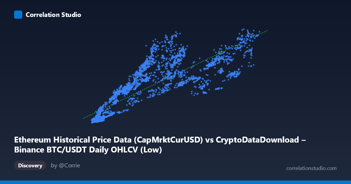
Ethereum Historical Price Data (CapMrktCurUSD) vs CryptoDataDownload – Binance BTC/USDT Daily OHLCV (Low)
- Pearson correlation (r)
- 0.8464
- Spearman correlation
- 0.9124
- p-value
- 0
- Sample size (n)
- 3191
- 95% confidence interval
- 0.8363 to 0.856
- Granger causality
- None
- Granger optimal lag
- 10
AI analysis
Analysis: Ethereum Market Cap vs. Bitcoin Price Relationship
Note on labeling: The axis metadata appears mismatched with the described columns (X labeled as Ethereum market cap, Y labeled as BTC/USDT Low price), but based on the data ranges and typical crypto market structure, this is best interpreted as a relationship between two crypto-market-linked variables — likely BTC price (X) and ETH market cap (Y), given X's range (~2,800–123,000) aligns with historical BTC price and Y's range (~$8.6B–$584B) aligns with ETH market capitalization.
1. Overall Relationship
The scatterplot reveals a strong positive, roughly linear relationship between the two variables. As X increases, Y increases in a consistent, monotonic fashion across nearly the entire observed range. The regression line (y = 4.116×10⁶x + 4.724×10¹⁰) fits the data reasonably well, though visible scatter around the line — especially at higher X values — suggests the relationship is not perfectly deterministic.
2. Strength, Direction, and Uncertainty
The correlation coefficient (r = 0.846) indicates a strong positive association, with r² = 0.716 meaning roughly 72% of the variance in Y is explained by X — a substantial but not complete explanatory relationship, leaving ~28% of variance driven by other factors. The 95% confidence interval [0.836, 0.856] is tight, and with p ≈ 0 across 3,191 paired observations, we can be highly confident this correlation is not due to chance. However, correlation does not imply causation here: the Granger causality tests show no significant predictive direction in either direction (X→Y: p = 0.664; Y→X: p = 0.757). This is a critical finding — despite the strong contemporaneous correlation, neither variable's past values help forecast the other's future values at the tested lag structure (10 periods). This strongly suggests both variables are driven by a common underlying factor (e.g., overall crypto market sentiment, liquidity cycles, or macro conditions) rather than one causing the other.
3. Notable Patterns and Outliers
The data shows a fan-shaped or heteroscedastic pattern — variance in Y appears to increase as X increases, particularly noticeable in the upper range (X 80,000), where Y values scatter more widely (e.g., X≈98,657 → Y≈482B vs. X≈109,977 → Y≈518B vs. X≈89,314 → Y≈379B). At low X values (< 10,000), points cluster tightly near the origin with less relative spread. There also appear to be two loose regimes: a lower-price cluster (X < 20,000) with proportionally lower Y values, and a higher-price cluster (X 50,000) where Y values are substantially elevated but more volatile — possibly reflecting distinct bull/bear market regimes rather than continuous scaling.
4. Confounding Factors and Caveats
Both variables are crypto-market-linked, meaning they likely share exogenous macro drivers: overall market liquidity, regulatory news, Bitcoin dominance cycles, stablecoin flows, and speculative sentiment. This creates a classic spurious/common-cause correlation risk — the strong r² may largely reflect shared exposure to crypto market cycles rather than a direct mechanical link between the two specific metrics. Additionally, the data spans 2017–2026, covering multiple boom-bust cycles (2017-18 bubble, 2021 bull run, 2022 crash, subsequent recovery), meaning the relationship is not stationary — its strength and slope likely vary significantly by market regime, which a single pooled r² does not capture.
5. Actionable Insights
1. Verify axis labeling — the metadata mismatch should be resolved before drawing firm conclusions about which specific variables are being compared. 2. Segment by market regime (bull vs. bear cycles) to check if the linear relationship holds consistently or if slope/r² shifts materially across periods. 3. Given the lack of Granger causality, avoid using one variable to forecast the other; instead, investigate shared upstream drivers (e.g., BTC dominance, total crypto market cap, macro liquidity indices) as better causal candidates. 4. Test for non-linear models (e.g., log-log regression) given the heteroscedasticity — crypto valuations often scale multiplicatively rather than additively, and a power-law fit may explain variance better than the linear model shown. 5. Extend lag structure in Granger tests beyond 10 periods, or test at different frequencies (weekly/monthly), since crypto markets may exhibit longer-horizon lead-lag relationships not captured at the current lag depth.
X dataset: CryptoDataDownload – Binance BTC/USDT Daily OHLCV
Y dataset: Ethereum Historical Price Data
Part of experiment: Bitcoin - CryptoDataDownload – Binance BTC/USDT Daily OHLCV vs Ethereum Historical Price Data