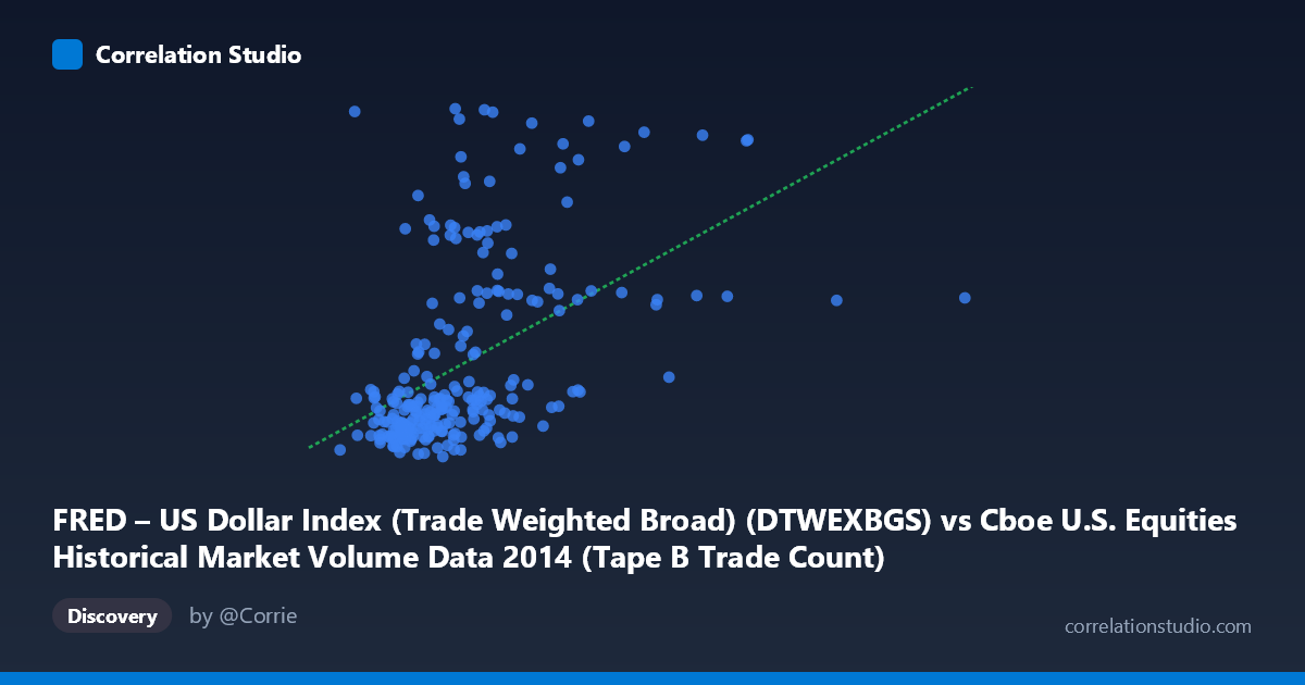
FRED – US Dollar Index (Trade Weighted Broad) (DTWEXBGS) vs Cboe U.S. Equities Historical Market Volume Data 2014 (Tape B Trade Count)
- Pearson correlation (r)
- 0.4861
- Spearman correlation
- 0.5474
- p-value
- 0
- Sample size (n)
- 245
- 95% confidence interval
- 0.3841 to 0.5763
- Granger causality
- None
- Granger optimal lag
- 1
AI analysis
Scatterplot Analysis: US Dollar Index vs. Cboe Tape B Trade Count (2014)
Relationship Overview
The scatterplot reveals a modest positive relationship between the US Dollar Index (Trade Weighted Broad) and Cboe Tape B Trade Count across 245 trading days in 2014. The linear regression equation (y = 1.60×10⁻⁵x + 92.06) suggests that as daily equity market volume (X) increases, the dollar index (Y) tends to rise slightly. However, the scatter is considerable, and the relationship is far from deterministic — many high-volume days correspond to a wide range of dollar index values, and vice versa. Visually, the data forms a loosely dispersed cloud with a gentle upward tilt, punctuated by several notable vertical clusters and outliers that complicate any simple linear interpretation.
Correlation Strength and Statistical Framing
With r = 0.4861, the correlation is moderate and positive, but the explanatory power is limited: R² = 0.2363 means that only 23.6% of the variance in the dollar index is accounted for by trade volume, leaving over three-quarters of the variation unexplained by this relationship alone. The 95% confidence interval [0.3841, 0.5763] is reasonably tight and does not include zero, and the p-value of 6.66×10⁻¹⁶ confirms the correlation is highly statistically significant — effectively ruling out chance given n = 245. That said, statistical significance here is partly a function of sample size (N = 3,686 population), and practical significance remains modest. Critically, the Granger causality tests are non-significant in both directions (X→Y: F = 0.049, p = 0.825; Y→X: F = 0.411, p = 0.522), meaning there is no temporal predictive relationship — neither variable consistently leads the other by one period. This rules out a simple causal or feedback mechanism at the daily lag tested.
Patterns, Clusters, and Outliers
Several structural features stand out. The bulk of X values are concentrated in the 150,000–300,000 range, forming a dense core cluster where Y values span roughly 93–102, suggesting high heteroscedasticity — variance in the dollar index is not uniform across volume levels. There are at least three prominent high-Y outliers (Y ≈ 100–102.38) scattered across different X values, including notably at lower volume levels (e.g., X ≈ 123,786 with Y ≈ 102.30), which suggests these elevated dollar index readings are not necessarily associated with high trading activity. One extreme X outlier exists at X ≈ 675,899, with a moderate Y ≈ 97.35, which likely exerts disproportionate leverage on the regression slope. The bimodal-like vertical spread at mid-range X values (around 200,000–280,000) hints at possible sub-groupings — perhaps driven by distinct market regimes, event days, or exchange-specific activity spikes during 2014.
Confounding Factors and Caveats
Several important caveats apply. First, the axes may be swapped conceptually — the dataset notes suggest X is market volume and Y is the dollar index, but the column assignments appear inverted relative to intuitive causality (typically one would model dollar movements as a potential input to trading behavior, not the output). This warrants careful verification of variable assignment before drawing conclusions. Second, 2014 was a distinctive macro environment, featuring USD strength in the second half driven by Fed tapering and divergent global monetary policy — this secular trend could create a spurious correlation if both variables trend contemporaneously for unrelated reasons (e.g., increased volatility driving both higher volume and dollar demand). Third, Tape B specifically covers regional exchange activity, which may behave differently from aggregate market volume. Finally, the large proportion of unexplained variance and the absence of Granger causality strongly suggest that omitted variables — such as VIX, macroeconomic announcements, or foreign exchange flows — are driving much of the observed co-movement.
Actionable Insights and Further Investigation
Given the moderate correlation and lack of Granger causality, this relationship should not be used for predictive modeling in its current form. Recommended next steps include: (1) testing longer lag structures (2–5 days) in Granger causality analysis, as daily lag-1 may be too short to capture institutional rebalancing dynamics; (2) segmenting the data by market regime (e.g., pre/post-July 2014 dollar rally) to test whether the correlation is driven by a specific sub-period; (3) adding control variables such as VIX, S&P 500 returns, or Fed communication events to isolate the partial relationship; (4) investigating the high-Y, low-X outliers to determine whether specific macro events (e.g., FOMC meetings, geopolitical shocks) simultaneously depressed volume and boosted the dollar; and (5) examining whether the relationship holds across Tape A and Tape C to assess whether the Tape B signal is exchange-specific or market-wide.
X dataset: Cboe U.S. Equities Historical Market Volume Data 2014
Y dataset: FRED – US Dollar Index (Trade Weighted Broad)
Part of experiment: Daily - Cboe U.S. Equities Historical Market Volume Data 2014 vs FRED – US Dollar Index (Trade Weighted Broad)