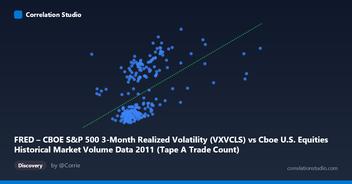
FRED – CBOE S&P 500 3-Month Realized Volatility (VXVCLS) vs Cboe U.S. Equities Historical Market Volume Data 2011 (Tape A Trade Count)
- Pearson correlation (r)
- 0.5089
- Spearman correlation
- 0.6169
- p-value
- 0
- Sample size (n)
- 252
- 95% confidence interval
- 0.4112 to 0.5951
- Granger causality
- None
- Granger optimal lag
- 1
AI analysis
Analysis of CBOE S&P 500 3-Month Realized Volatility vs. Tape A Trade Count (2011)
1. What the Visualization Reveals
The scatterplot depicts the relationship between CBOE S&P 500 3-Month Realized Volatility (VXVCLS) on the X-axis and Tape A Trade Count from U.S. equities market volume data on the Y-axis across 252 trading days in 2011. The overall pattern shows a positive, moderately dispersed relationship: as realized volatility rises, trade counts tend to increase as well. However, the relationship is far from clean — a wide band of scatter is visible across the full range of X values, and there appears to be a notable concentration of points at lower volatility levels with a thinning, upward-stretching tail at higher volatility readings, suggesting the relationship may be non-linear or heteroscedastic in nature.
2. Correlation Strength, Direction, and Statistical Framing
The Pearson correlation of r = 0.509 indicates a moderate positive association, but the explanatory power is limited: r² = 0.259, meaning realized volatility accounts for only about 26% of the variance in Tape A trade counts, leaving roughly three-quarters of the variation unexplained by this single predictor. The 95% confidence interval of [0.411, 0.595] is meaningfully above zero and relatively tight given the sample size (n = 252), and the p-value of effectively 0 confirms this association is highly statistically significant — not a sampling artifact. That said, statistical significance does not imply practical sufficiency. Critically, the Granger causality tests fail in both directions (X→Y: F = 0.0001, p = 0.99; Y→X: F = 0.173, p = 0.68), meaning neither variable temporally predicts the other with a one-period lag. This is an important caveat: while the two variables move together contemporaneously, there is no evidence that past volatility readings predict future trade volume, or vice versa. The relationship appears to be coincident rather than predictive.
3. Notable Patterns, Clusters, and Outliers
Several structural features stand out in the data. First, there is a dense cluster of observations at lower volatility values (roughly 17–22 on Y, concentrated in the 900,000–1,200,000 X range), suggesting that the majority of 2011 trading days were characterized by moderate, relatively stable conditions. Second, a distinct upper tail emerges — a handful of points reach trade counts of 35–43, associated with higher volatility readings — consistent with well-known volatility spikes during the European debt crisis and U.S. debt ceiling debates of mid-to-late 2011. Third, one point near X ≈ 2,126,542 with Y ≈ 33.8 appears as a high-leverage outlier far to the right of the main distribution, potentially representing an extreme market stress day. The observation that Spearman ρ exceeds Pearson r confirms that the relationship is better described by a monotonic but non-linear function — a logarithmic or polynomial fit would likely capture the curvature in the upper range more accurately than the fitted linear model (y = 1.117×10⁻⁵x + 12.02).
4. Confounding Factors and Caveats
Several important caveats temper interpretation. First, both variables are driven by common macroeconomic shocks — major geopolitical or financial events simultaneously elevate volatility and trading activity, creating a spurious appearance of direct causation when both are downstream of a shared third factor (e.g., the 2011 sovereign debt crisis). Second, market structure effects such as algorithmic trading, exchange fee changes, or fragmentation across venues could independently drive Tape A trade counts without any relationship to volatility levels. Third, the linear regression's residual 74% unexplained variance and the non-linearity signal suggest that important explanatory variables are omitted — liquidity conditions, options market activity, and institutional rebalancing cycles are plausible candidates. Finally, the time series nature of the data means observations are not truly independent, and standard correlation assumptions may be violated even though Granger causality found no lag-1 predictive structure.
5. Actionable Insights and Further Investigation
Given the moderate but incomplete correlation and the absence of Granger causality, practitioners should avoid using volatility alone as a trading volume predictor for operational or liquidity planning purposes. Several next steps are warranted: (a) Fit a logarithmic or polynomial regression to better capture the apparent non-linearity, particularly in the high-volatility tail; (b) Test longer Granger causality lags (2–5 periods) to rule out delayed predictive relationships; (c) Disaggregate the analysis by market regime (low vs. high volatility periods) to assess whether the correlation strengthens meaningfully during stress episodes; (d) Introduce multivariate controls such as VIX level, bid-ask spreads, or macro event indicators to isolate the marginal contribution of realized volatility; and (e) Examine whether the extreme outlier near X ≈ 2.1M represents a data quality issue or a genuine structural break warranting separate treatment in any predictive model.
X dataset: Cboe U.S. Equities Historical Market Volume Data 2011
Y dataset: FRED – CBOE S&P 500 3-Month Realized Volatility
Part of experiment: Daily - Cboe U.S. Equities Historical Market Volume Data 2011 vs FRED – CBOE S&P 500 3-Month Realized Volatility