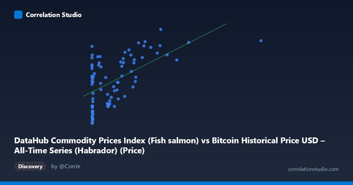
DataHub Commodity Prices Index (Fish salmon) vs Bitcoin Historical Price USD – All-Time Series (Habrador) (Price)
- Pearson correlation (r)
- 0.5838
- Spearman correlation
- 0.5206
- p-value
- 0
- Sample size (n)
- 83
- 95% confidence interval
- 0.4211 to 0.7101
- Granger causality
- None
- Granger optimal lag
- 1
- Time coverage
- 2010-08-01 to 2017-06-01
- Recomputed on refreshed data
- 2026-10-24 (r was 0.5838)
AI analysis
Analysis: Bitcoin Price vs. Fish Salmon Commodity Index
1. What the Visualization Reveals
The scatterplot shows a moderate positive relationship between Bitcoin's historical USD price (X) and a fish/salmon commodity price index (Y). The data reveals a clear non-linear, logarithmic-like pattern rather than a strictly linear one: Y rises steeply as X moves from near-zero to a few hundred dollars, then the rate of increase flattens considerably as X climbs into the thousands. This is consistent with the extreme right-skew in X (mean $321 vs. stdev $405, range up to $2,452), which compresses most low-price Bitcoin observations into a narrow band while a handful of high-price points stretch the axis.
2. Strength, Direction, and Uncertainty
The correlation coefficient (r = 0.584) indicates a moderate positive linear association, with r² = 0.341 meaning only about 34% of the variance in the commodity index is statistically explained by Bitcoin's price — leaving nearly two-thirds of the variance attributable to other factors. The 95% CI [0.421, 0.710] is reasonably tight and entirely positive, and the p-value (6.9×10⁻⁹) confirms this correlation is highly unlikely due to chance. However, correlation strength here should not be overstated: r=0.58 is "moderate," not strong, and the relationship is likely better fit by a non-linear model given the visual curvature. Critically, the Granger causality tests show no significant predictive direction in either direction (X→Y: p=0.877; Y→X: p=0.107, though the latter is closer to significance). This means neither series reliably helps forecast the other's future values — the association is contemporaneous/structural rather than causal or lead-lag in nature.
3. Notable Patterns and Outliers
Several clusters stand out: a dense cluster of low-X points (X < 20) with Y ranging widely from ~4.2 to ~7.8, suggesting high variance in the commodity index during Bitcoin's earliest, lowest-price era. A middle cluster (X: 100–700) shows Y climbing steadily from ~5 to ~7.5. At the high end (X 900), Y plateaus around 7.2–8.6, suggesting diminishing marginal association. Notable outliers include points like (0.77, 7.84), (3.03, 7.43), and (0.92, 7.30) — very low Bitcoin prices paired with unexpectedly high index values — which don't fit the general upward trend and may reflect early-period volatility or data artifacts.
4. Confounding Factors and Caveats
This is a classic case of spurious correlation via shared time trend. Both series are time-indexed from 2010–2017, and Bitcoin's price grew by orders of magnitude over this period (a global secular trend), while commodity/food indices also drifted upward due to unrelated macroeconomic inflation, seasonal fishing yields, or global food price cycles. Two unrelated trending time series will often show statistically significant correlation without any causal link — a well-known pitfall (Granger's original "spurious regression" concern). The lack of Granger causality in either direction strongly supports this interpretation: there's no mechanistic pathway connecting Bitcoin adoption/speculation to salmon pricing. Additionally, n=83 paired points sampled from N=449 possible observations, and the non-normal, heavy-tailed distribution of X (stdev roughly equals mean) violates linear regression assumptions.
5. Actionable Insights
Given the mismatched, likely coincidental variable pairing (Bitcoin price vs. fish commodity index), this correlation should not be used for trading, forecasting, or hedging strategies. To properly test any relationship, analysts should: (a) detrend both series (e.g., using first differences or log-returns) and re-run the correlation to check if it evaporates — a strong diagnostic for spurious trend correlation; (b) consider log-transforming X given its skew, which may better linearize the visible curvature and improve model fit; and (c) explore whether both series are merely proxies for a common macro factor (e.g., USD strength/inflation) rather than testing them against each other directly.
X dataset: Bitcoin Historical Price USD – All-Time Series (Habrador)
Y dataset: DataHub Commodity Prices Index
Part of experiment: Bitcoin - Bitcoin Historical Price USD – All-Time Series (Habrador) vs DataHub Commodity Prices Index