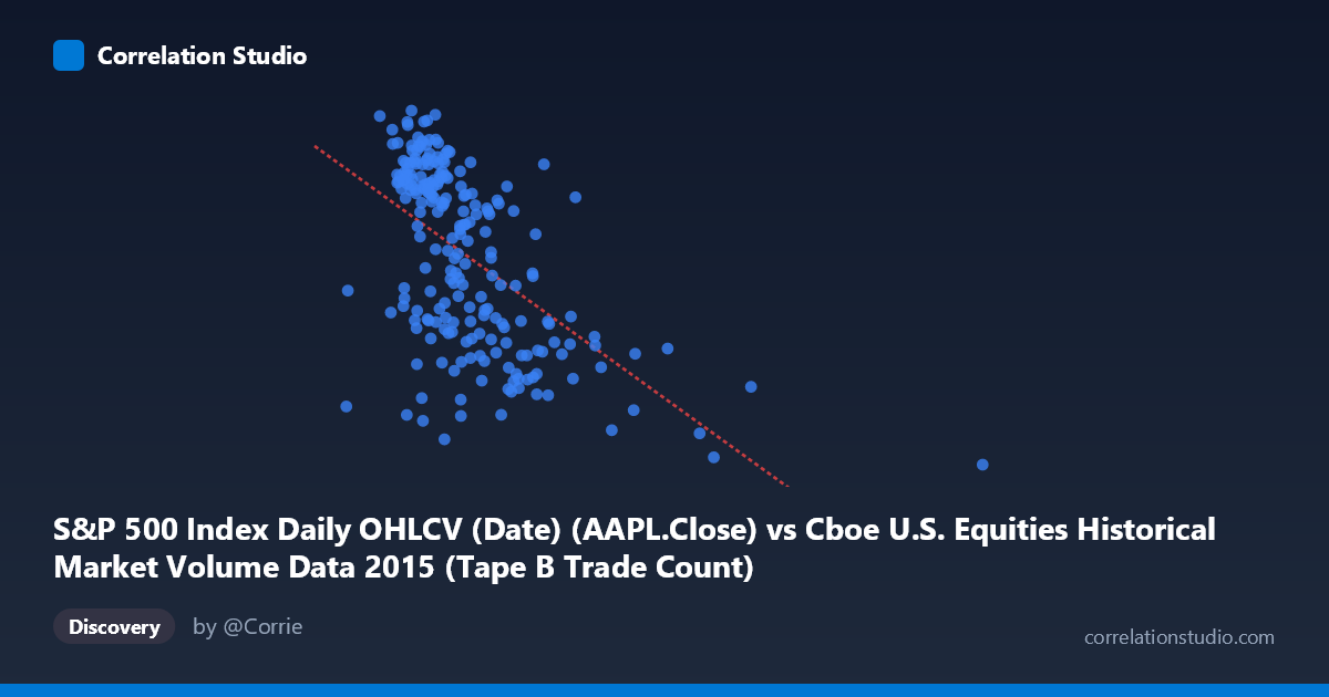
S&P 500 Index Daily OHLCV (Date) (AAPL.Close) vs Cboe U.S. Equities Historical Market Volume Data 2015 (Tape B Trade Count)

Pearson correlation (r): -0.565
Spearman correlation: -0.6024
p-value: 0
Sample size (n): 222
95% confidence interval: -0.6484 to -0.4681
Granger causality: None
Granger optimal lag: 1

AI analysis

Scatterplot Analysis: AAPL Close Price vs. Cboe Tape B Trade Count (2015)

Relationship Overview The scatterplot reveals a negative relationship between Apple's closing stock price (X-axis) and the Cboe U.S. Equities Tape B Trade Count (Y-axis) over 2015. As AAPL's price increases, the Tape B trade count tends to decrease, and vice versa. The linear regression equation (y = -4.38×10⁻⁵x + 133.773) confirms this downward slope, suggesting that higher AAPL valuations are associated with fewer Tape B trades. Visually, the bulk of data points cluster in the lower-left region (AAPL prices roughly $200K–$400K range with trade counts between 110–133), with the relationship becoming more apparent at the extremes.

Correlation Strength and Statistical Significance The Pearson correlation of r = -0.565 indicates a moderate negative association, but the explanatory power is more modest than the coefficient alone implies — r² = 0.319 means only ~32% of the variance in Tape B trade counts is explained by AAPL's closing price. The remaining ~68% is attributable to other factors entirely. The 95% confidence interval of [-0.648, -0.468] is relatively narrow and does not cross zero, and the p-value is effectively zero (p < 0.001, n = 222), confirming this relationship is highly statistically significant and unlikely to be a sampling artifact. However, statistical significance should not be conflated with practical or causal significance. Critically, the Granger causality tests show no significant predictive directionality in either direction (X→Y: F = 1.42, p = 0.234; Y→X: F = 0.07, p = 0.793), meaning that past values of AAPL price do not meaningfully help forecast future Tape B trade counts, and vice versa. This decouples any temporal predictive utility from the observed contemporaneous correlation.

Notable Patterns, Clusters, and Outliers Three distinct features stand out. First, the primary cluster sits tightly between X ≈ 130,000–450,000 and Y ≈ 103–133, showing moderate scatter consistent with the r² value. Second, there are two pronounced outliers pulling the regression strongly: one point near (1,014,195, 103.12) and another near (640,679, 103.74), both representing days with unusually high AAPL closing values and exceptionally low trade counts. These extreme observations disproportionately influence the regression slope and correlation coefficient. Third, within the main cluster, the relationship appears somewhat non-linear or heteroscedastic — variance in Y is larger at moderate X values and compresses at the extremes — suggesting a simple linear model may be an oversimplification of the true relationship.

Confounding Factors and Caveats Several important caveats apply. The axis labels appear to be swapped based on the dataset descriptions (AAPL Close is listed as the X variable from the Cboe dataset, and Tape B Trade Count is the Y variable from the S&P 500 dataset), which warrants careful verification before drawing conclusions. More fundamentally, the negative correlation almost certainly reflects a shared temporal driver: AAPL's price declined significantly in mid-to-late 2015, while market volatility and trading volume (including Tape B) surged during the same period, particularly around the August 2015 market correction. This means both variables are likely responding to macroeconomic and market stress conditions rather than causally influencing each other. Additionally, Tape B covers NYSE American and regional exchanges, which may respond to broad market conditions differently than AAPL-specific dynamics.

Actionable Insights and Further Investigation Given the absence of Granger causality, using AAPL price alone as a predictor of Tape B trade count in a trading or operational model would be inadvisable. Instead, analysts should: (1) test whether the correlation is spurious by controlling for market-wide volatility indices (e.g., VIX) or overall market volume as potential common drivers; (2) investigate the two extreme outliers to determine if they represent data entry errors, corporate events, or genuine market anomalies, as removing them may substantially change the regression; (3) explore non-linear modeling (e.g., log-transforming X, or applying a polynomial fit) given the apparent heteroscedasticity; and (4) extend the time series beyond 2015 to assess whether this relationship is stable or specific to that year's unusual market conditions, particularly the August correction.

X dataset: Cboe U.S. Equities Historical Market Volume Data 2015

Y dataset: S&P 500 Index Daily OHLCV (Date)

Part of experiment: Daily - Cboe U.S. Equities Historical Market Volume Data 2015 vs S&P 500 Index Daily OHLCV (Date)