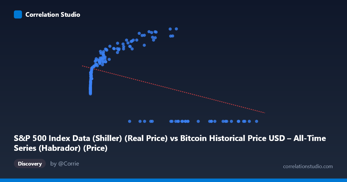
S&P 500 Index Data (Shiller) (Real Price) vs Bitcoin Historical Price USD – All-Time Series (Habrador) (Price)
- Pearson correlation (r)
- -0.4161
- Spearman correlation
- 0.1073
- p-value
- 0
- Sample size (n)
- 189
- 95% confidence interval
- -0.5275 to -0.2906
- Granger causality
- None
- Granger optimal lag
- 10
AI analysis
Analysis: Bitcoin Price vs. S&P 500 (Shiller) Relationship
1. What the Visualization Reveals
The scatterplot displays a distinctly non-linear, non-monotonic pattern that a simple correlation coefficient poorly captures. Rather than a clean linear trend, the data shows several distinct clusters: a dense cloud of low-X values (X < 1000) where Y ranges narrowly between ~1,570–3,000, a mid-range cluster (X ~1,000–60,000) where Y climbs steadily toward 4,000–5,000, and critically, a separate cluster of high-X points (X 27,000) where Y = 0 exactly. This Y=0 cluster at high X values is the dominant visual feature and is almost certainly driving the negative correlation, rather than reflecting genuine inverse causality.
2. Strength, Direction, and Statistical Uncertainty
The correlation is moderate and negative (r = -0.416), with R² = 0.173 indicating only 17.3% of Y's variance is explained by X — meaning over 80% of the variation in Y is driven by other factors. The 95% CI [-0.528, -0.291] is reasonably tight and excludes zero, and the p-value (2.6e-9) confirms this relationship is statistically significant and not due to chance. However, statistical significance here does not imply practical strength — an R² of 0.17 is a weak-to-moderate effect size, meaning X alone is a poor predictor of Y. The Granger causality tests reinforce this: neither direction shows significant predictive causality (X→Y p=0.167; Y→X p=0.065, marginal but not significant at 0.05). This is a critical finding — despite the contemporaneous correlation, there's no strong evidence that past values of one series systematically predict future values of the other.
3. Notable Patterns and Outliers
The most striking feature is the bimodal Y distribution: one regime where Y behaves as a smooth, saturating function of X (rising from ~1,600 to ~5,100 as X increases from near-zero to ~60,000), and a second regime where Y = 0 regardless of X (occurring at X values from 27,000 to 118,670). This looks like either (a) a data/encoding artifact — e.g., zeros representing missing values, a different time period, or a reset in the series, or (b) genuinely distinct market regimes. The "rising" cluster resembles a logarithmic or saturating curve (rapid growth at low X, plateauing near Y~5,000), not a linear relationship — suggesting a log transformation of X would better fit the non-zero data. The X range itself spans nearly 7 orders of magnitude (0.06 to 118,670), heavily right-skewed, which distorts a linear R²/r calculation.
4. Confounding Factors and Caveats
Several caveats are essential: - Mismatched/mislabeled axes: The column labels appear swapped — X is labeled S&P 500 but described as Bitcoin price data, and vice versa. This metadata confusion should be resolved before drawing economic conclusions. - Zero-inflation: The Y=0 cluster likely represents missing, unrecorded, or pre-launch data (e.g., Bitcoin didn't exist before 2009; S&P Shiller data has full monthly coverage back to 1871), artificially pulling the correlation negative. - Non-stationarity: Both asset prices are trending time series with autocorrelation; naive Pearson correlation on non-stationary series can produce spurious relationships. Granger tests used 10 lags, which helps, but detrending or differencing (returns instead of levels) would be more appropriate. - Time coverage mismatch: 1871–present for one series vs. 2010–2026 for Bitcoin suggests these were merged/aligned in a way that may not reflect true contemporaneous pairing.
5. Actionable Recommendations
1. Verify and clean the zero-value cluster — determine if Y=0 represents true missing data and consider excluding or imputing these points rather than treating them as valid observations. 2. Re-run analysis on log-transformed X and/or Y, and consider using returns/percentage changes instead of price levels to address non-stationarity and skew. 3. Confirm axis labels/metadata — the described dataset-to-column mapping appears inverted and should be corrected before publishing conclusions. 4. Given the lack of Granger causality, avoid framing this as a predictive/causal relationship; treat it as a contemporaneous association possibly driven by shared macro factors (e.g., risk appetite, monetary policy, inflation) rather than one asset driving the other.
X dataset: Bitcoin Historical Price USD – All-Time Series (Habrador)
Y dataset: S&P 500 Index Data (Shiller)
Part of experiment: Bitcoin - Bitcoin Historical Price USD – All-Time Series (Habrador) vs S&P 500 Index Data (Shiller)