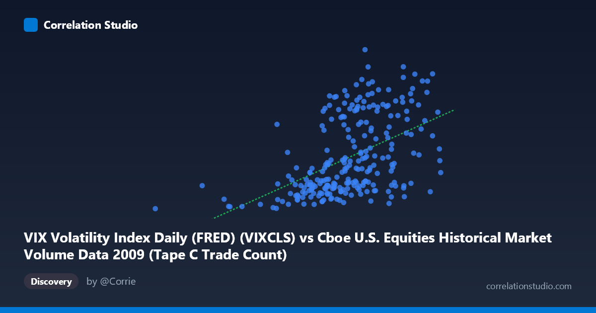
VIX Volatility Index Daily (FRED) (VIXCLS) vs Cboe U.S. Equities Historical Market Volume Data 2009 (Tape C Trade Count)
- Pearson correlation (r)
- 0.5002
- Spearman correlation
- 0.5446
- p-value
- 0
- Sample size (n)
- 252
- 95% confidence interval
- 0.4014 to 0.5875
- Granger causality
- None
- Granger optimal lag
- 1
AI analysis
Analysis: VIX Volatility Index vs. Cboe Tape C Trade Count (2009)
Relationship Overview The scatterplot reveals a moderate positive relationship between the VIX Volatility Index and Cboe Tape C trade counts during 2009. As the VIX rises — indicating greater market fear and uncertainty — the number of trades on Tape C venues tends to increase. This is consistent with well-established market microstructure theory: elevated volatility typically drives higher trading activity as investors rebalance portfolios, hedge exposures, and react to rapidly changing prices. The linear regression equation (y = 4.54E-05x + 2.61) captures this upward trend, though the scatter around the line is considerable, immediately suggesting the relationship is real but far from deterministic.
Correlation Strength and Statistical Framing The Pearson correlation of r = 0.50 reflects a moderate positive association, but the more telling figure is r² = 0.25 — meaning VIX levels explain only about 25% of the variance in Tape C trade counts. Three-quarters of the variation in trading volume remains attributable to other factors entirely. The 95% confidence interval of [0.40, 0.59] is meaningfully above zero and reasonably tight given n = 252, and the p-value of effectively zero confirms this relationship is not a sampling artifact. However, despite statistical significance, the Granger causality tests are non-significant in both directions (X→Y: F = 0.45, p = 0.50; Y→X: F = 0.03, p = 0.85), meaning neither variable reliably predicts the other at a one-period lag. This is a critical caveat: while VIX and trade counts co-move, there is no evidence of a clean temporal lead-lag predictive relationship at daily frequency.
Notable Patterns and Outliers The sample points reveal meaningful clustering and heterogeneity. A dense cluster sits in the lower-left region — VIX values roughly between 500,000–650,000 and trade counts in the 20–30 range — likely corresponding to calmer mid-to-late 2009 periods as markets stabilized post-crisis. A second, more dispersed cluster occupies the upper range, with several points exceeding trade counts of 40–52 (e.g., (679,961, 52.62) and (761,867, 52.65)), coinciding with elevated VIX readings. Notably, the point (185,886, 19.47) stands out as a clear outlier on the low end of both axes, potentially representing an anomalous low-volume, low-volatility day early in the year. The spread of trade counts at any given VIX level is wide — for example, VIX values near 650,000–700,000 produce trade counts ranging from ~22 to ~53 — suggesting substantial conditional variance that a simple linear model cannot capture.
Confounding Factors and Caveats Several important caveats apply. First, 2009 is a highly unusual year — it spans the tail end of the Global Financial Crisis and the subsequent recovery rally, meaning the VIX-volume relationship may be regime-dependent rather than generalizable. Second, Tape C trade count captures only a subset of U.S. equity trading, and routing decisions between venues introduce noise unrelated to volatility. Third, day-of-week effects, earnings seasons, index rebalancing events, and macroeconomic announcements all drive trading activity independently of VIX. Fourth, the non-significant Granger results suggest contemporaneous co-movement may be driven by a common external driver (e.g., macroeconomic news shocks) rather than a direct causal pathway between VIX and trade counts. Finally, treating N = 3,232 as the population while sampling n = 252 is appropriate, but daily financial time series exhibit autocorrelation, which can inflate effective sample sizes and overstate precision.
Actionable Insights and Further Investigation Practitioners and researchers should consider several next steps. The 25% explained variance and non-significant Granger causality suggest that VIX alone is insufficient as a predictor of Tape C activity — incorporating additional regressors (e.g., realized volatility, bid-ask spreads, macro surprise indices) would likely improve explanatory power substantially. A regime-based or segmented analysis (e.g., separating Q1 crisis-period observations from Q3–Q4 recovery) could reveal whether the correlation strengthens or weakens across market states. Testing non-linear specifications (e.g., log-log or spline regression) is warranted given the visual spread and potential floor effects at low VIX levels. For trading applications, investigating intraday VIX-volume dynamics or extending the dataset across multiple years would help assess whether this moderate correlation is structurally stable or a 2009-specific artifact of extraordinary market conditions.
X dataset: Cboe U.S. Equities Historical Market Volume Data 2009
Y dataset: VIX Volatility Index Daily (FRED)
Part of experiment: Daily - Cboe U.S. Equities Historical Market Volume Data 2009 vs VIX Volatility Index Daily (FRED)