Cboe U.S. Equities Historical Market Volume Data 2025 (Tape B Trade Count) vs Brent Daily Spot Prices (Price)
- Pearson correlation (r)
- -0.4017
- Spearman correlation
- -0.4566
- p-value
- 0
- Sample size (n)
- 246
- 95% confidence interval
- -0.5016 to -0.2912
- Granger causality
- None
- Granger optimal lag
- 10
AI analysis
Scatterplot Analysis: Brent Crude Oil Prices vs. Cboe Tape B Trade Count (2025)
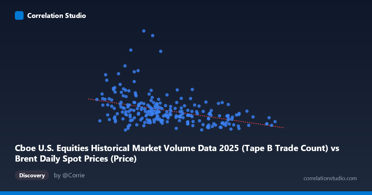
Relationship Overview The scatterplot reveals a modest negative relationship between Cboe U.S. Equities Tape B trade counts (X-axis, ranging ~60–83 units) and daily Brent crude oil spot prices (Y-axis, ranging ~$407K–$1.72M in the scaled units shown). The linear regression line (y = -14,758.9x + 1,686,290) slopes downward, suggesting that on days when equity trade counts are higher, Brent crude prices tend to be somewhat lower. However, the scatter around this line is considerable, and a handful of extreme values dominate the visual impression of the relationship.
Correlation Strength and Statistical Significance The Pearson correlation of r = -0.40 indicates a weak-to-moderate negative association. Critically, r² = 0.161, meaning that Tape B trade count explains only about 16% of the variance in Brent crude prices — leaving 84% attributable to other factors entirely. The 95% confidence interval of [-0.50, -0.29] is reasonably tight and does not cross zero, and the p-value of 5.9×10⁻¹¹ confirms this correlation is highly statistically significant given the large population (N = 4,805) and sample size (n = 246). However, statistical significance here is partly a function of sample size and should not be mistaken for practical or economic significance. Most importantly, the Granger causality tests show no significant directional predictive relationship in either direction (X→Y: p = 0.82; Y→X: p = 0.56), meaning neither variable reliably predicts the other temporally — the correlation is contemporaneous at best, not mechanistically directional.
Notable Patterns, Clusters, and Outliers Several features stand out in the data. There is a dense central cluster of points between X ≈ 63–74 and Y ≈ $450K–$800K, forming the bulk of the distribution. At least two prominent high-Y outliers are visible — most notably the point at approximately (66.13, 1,718,887) and another near (64.86, 1,178,999) and (62.78, 1,152,125) — which exert disproportionate leverage on the regression line and likely inflate the apparent negative slope. On the high-X end, the point at (83.48, 517,437) is a clear univariate outlier in X, isolated well beyond the main cluster. These outliers suggest the relationship may not be as cleanly linear as the model implies, and their removal could materially change r.
Confounding Factors and Interpretive Caveats A fundamental caveat is that the dataset labels appear to be cross-applied: the X-axis is labeled as Tape B trade counts from a Brent crude dataset, and the Y-axis as Brent prices from a Cboe dataset — suggesting these are two distinct data series that have been paired by date rather than being causally linked instruments. Any observed correlation could easily be spurious co-movement driven by shared temporal trends (e.g., macroeconomic conditions in 2025, risk-on/risk-off regimes, or calendar effects). The lack of Granger causality at up to 10 lags reinforces this interpretation. Additionally, the high-Y outliers could reflect data quality issues, unit inconsistencies, or exceptional market events rather than genuine signal.
Actionable Insights and Further Investigation Given the weak explanatory power and absence of Granger causality, this correlation should not be used as a trading or forecasting signal in isolation. Recommended next steps include: (1) removing or investigating the high-leverage outliers to determine whether they reflect data errors or genuine events; (2) controlling for date-based confounders such as day-of-week effects, macro announcements, or volatility regimes using multivariate regression; (3) testing non-linear specifications (e.g., polynomial or quantile regression) given the apparent heteroscedasticity in the scatter; and (4) cross-referencing with broader market variables (VIX, USD index, crude inventory data) to identify whether any three-way relationship explains both series simultaneously. The 2025-only time window also limits generalizability, and extending the analysis to multi-year data would help distinguish structural relationships from year-specific noise.
X dataset: Brent Daily Spot Prices
Y dataset: Cboe U.S. Equities Historical Market Volume Data 2025
Part of experiment: Daily - Brent Daily Spot Prices vs Cboe U.S. Equities Historical Market Volume Data 2025