US Car & Light Truck Retail Sales – Domestic (FRED DAUTOSAAR) (DAUTOSAAR) vs Our World in Data Air Passengers Carried (Air transport, passengers carried)
- Pearson correlation (r)
- -0.7836
- Spearman correlation
- -0.8266
- p-value
- 0
- Sample size (n)
- 54
- 95% confidence interval
- -0.8691 to -0.6529
- Granger causality
- None
- Granger optimal lag
- 1
AI analysis
Scatterplot Analysis: US Domestic Auto Sales vs. Global Air Passengers Carried
1. Overall Relationship
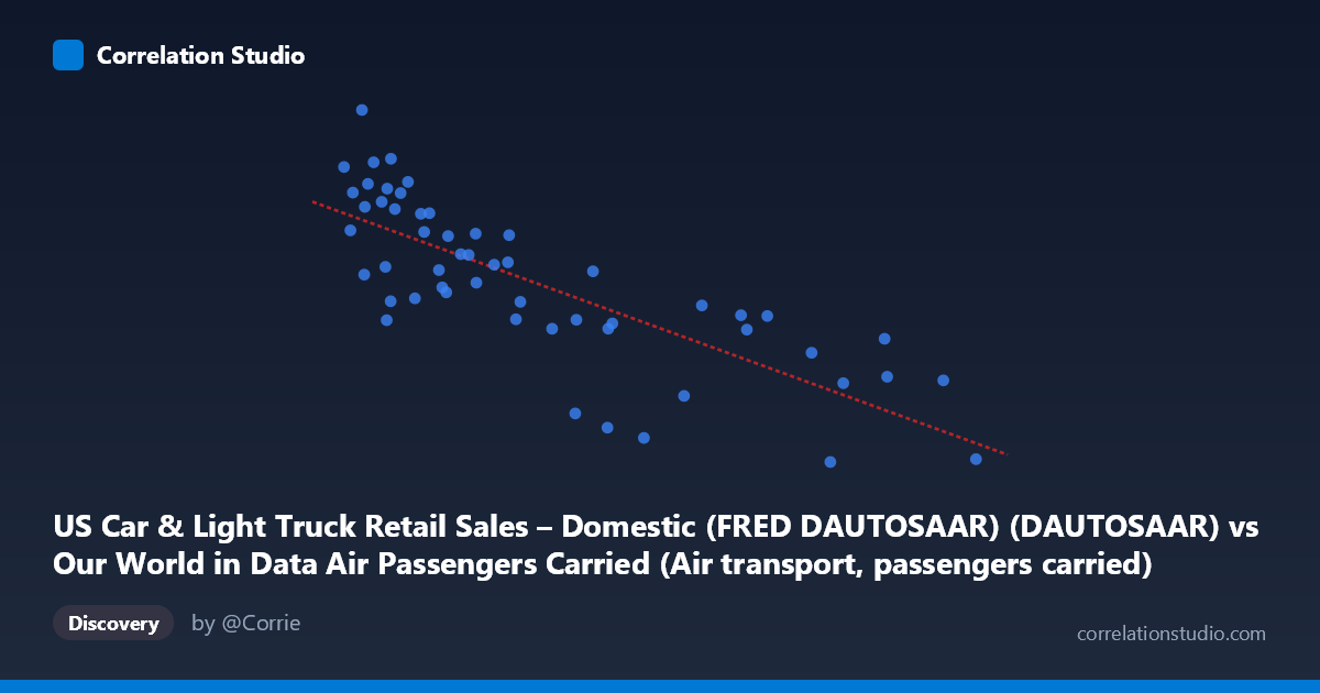
The scatterplot reveals a clear negative relationship between US domestic car and light truck retail sales (X-axis) and global air passengers carried (Y-axis). As domestic auto sales increase, air passenger volumes tend to decrease — and vice versa. The linear regression line (y = -4.15E-08x + 8.12) captures this downward trend reasonably well across the observed range, though considerable scatter around the line suggests the relationship is not perfectly linear. Visually, data points cluster more densely at lower X values (roughly 8M–40M units) with higher Y values, while higher X values correspond to notably lower air passenger figures, painting a coherent — if initially counterintuitive — picture across the 1970–2023 time span.
2. Correlation Strength, Direction, and Predictive Value
The Pearson correlation of r = -0.784 indicates a moderately strong negative association. The R² of 0.614 means that approximately 61.4% of the variance in air passengers carried is statistically explained by domestic auto sales levels — a substantial explanatory share for a social-science cross-domain relationship, but also a reminder that nearly 40% of variance remains unexplained by this single predictor. The 95% confidence interval of [-0.869, -0.653] is relatively tight and entirely negative, reinforcing confidence that the negative direction is genuine and not an artifact of sampling. The p-value of 2.46 × 10⁻¹² is extraordinarily small, confirming the correlation is highly statistically significant across the n=54 paired sample drawn from a population of N=712.
Critically, however, the Granger causality tests reveal no significant temporal predictive direction in either direction (X→Y: F=0.000, p=0.995; Y→X: F=2.15, p=0.149). This means that knowing past auto sales does not meaningfully improve forecasts of future air passengers, and vice versa. The correlation is therefore associative and likely driven by shared time-trends rather than any direct causal mechanism between the two variables.
3. Notable Patterns, Clusters, and Outliers
Several features merit attention:
- Lower-left cluster: Points around X = 8M–20M with Y values of 5.3–10.1 show considerable vertical spread, suggesting that at low auto sales volumes (likely corresponding to earlier decades or recession periods), air travel was more variable and generally higher in relative terms. - High-leverage outliers at high X: Points such as (105.2M, 2.11), (134.3M, 2.18), and (127.7M, 3.98) sit at the far right with very low Y values. These likely represent specific years (possibly around 2020–2021 COVID collapse in air travel, or specific auto-sales peak years) and exert strong influence on the regression slope. - Mid-range anomalies: (54.3M, 3.22), (75.98M, 3.62), and (60.69M, 2.90) fall noticeably below the regression line, indicating periods where air travel dropped sharply despite moderate auto sales — consistent with events like post-9/11 travel disruption or financial crises. - Point (11.67M, 10.14) is the highest Y-value observation, consistent with an early-decade period of strong air travel growth and lower auto sales volumes.
The scatter is somewhat heteroscedastic — variance in Y appears larger at low X values and compresses at high X — which mildly violates linear regression assumptions and suggests a potential log or power-law transformation might better fit the data.
4. Confounding Factors and Interpretive Caveats
This correlation almost certainly reflects shared temporal trends rather than a direct structural relationship between the two markets:
- Time as a lurking variable: Both series span 1970–2023. Over this period, air travel grew substantially through the 1990s–2000s before being disrupted by COVID-19, while domestic auto sales fluctuated with business cycles. The negative correlation may largely capture the fact that recent years saw COVID-19 devastate air travel while auto sales (seasonally adjusted) remained relatively high in pre- and post-pandemic context. - GDP and macroeconomic cycles: Both variables respond to economic conditions, but in potentially opposing ways depending on the period — recessions reduce auto sales but may also reduce air travel, which would attenuate rather than produce the negative correlation. - Structural market shifts: The rise of SUVs/light trucks in domestic sales, fuel price shocks, airline deregulation, and the emergence of low-cost carriers all independently influence each series across the timeframe. - Dataset mismatch: The X variable is specifically US domestic auto sales, while the Y variable appears to be global air passengers — this geographic mismatch means the correlation conflates US consumer behavior with worldwide aviation activity, dramatically limiting causal interpretability. - Seasonality and aggregation: Monthly auto sales data aggregated or sampled annually alongside annual air passenger data may introduce aggregation artifacts.
5. Actionable Insights and Further Investigation
Despite the statistical significance, the absence of Granger causality is the most actionable finding: analysts should not use domestic auto sales as a leading indicator for air travel demand (or vice versa) in forecasting models. The correlation is likely spurious at the causal level.
Recommended next steps include:
- Partial out time trends: Run a detrended or first-differenced regression to test whether the correlation persists once shared temporal drift is removed — this would be the most critical robustness check. - Restrict geographic scope: Replace global air passengers with US-specific domestic air passenger data to achieve a more apples-to-apples comparison and test whether a genuine substitution or complementarity effect exists. - Introduce control variables: Add GDP, fuel prices, and recession indicators as covariates to determine whether the auto–air correlation survives multivariate adjustment. - Investigate the COVID outliers: Isolate and analyze the 2019–2022 data points separately, as pandemic-era observations may be disproportionately driving the observed correlation. - Test non-linear specifications: Given the heteroscedastic scatter, a log-log or semi-log regression may yield better fit and more stable residuals across the full range of the data.
X dataset: Our World in Data Air Passengers Carried
Y dataset: US Car & Light Truck Retail Sales – Domestic (FRED DAUTOSAAR)
Part of experiment: Yearly - Our World in Data Air Passengers Carried vs US Car & Light Truck Retail Sales – Domestic (FRED DAUTOSAAR)