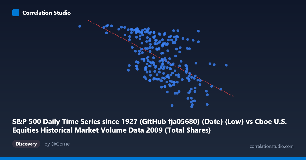
S&P 500 Daily Time Series since 1927 (GitHub fja05680) (Date) (Low) vs Cboe U.S. Equities Historical Market Volume Data 2009 (Total Shares)
- Pearson correlation (r)
- -0.5621
- Spearman correlation
- -0.554
- p-value
- 0
- Sample size (n)
- 252
- 95% confidence interval
- -0.6411 to -0.4712
- Granger causality
- X → Y
- Granger optimal lag
- 10
AI analysis
Analysis: S&P 500 Daily Low vs. Cboe Total Shares Traded (2009)
Relationship Overview The scatterplot reveals a moderate negative relationship between the S&P 500 daily low price and total shares traded on U.S. equities exchanges throughout 2009. The linear regression equation (y = -4.25×10⁻⁷x + 1,261.71) confirms that as the S&P 500 low price increases, total shares traded tend to decrease. This is visually consistent with a classic "fear-driven volume" dynamic: during the early 2009 period when index prices were depressed (near multi-year lows following the 2008 financial crisis), trading volumes were elevated, while as prices recovered through the year, volumes gradually normalized downward. The relationship, while statistically clear, shows considerable scatter, indicating this is a probabilistic tendency rather than a deterministic rule.
Correlation Strength and Statistical Significance The Pearson correlation of r = -0.5621 represents a moderate negative association, but the more meaningful metric is r² = 0.3159, meaning that S&P 500 daily low prices explain only about 31.6% of the variance in total shares traded. The remaining ~68% of variability in trading volume is driven by other factors entirely. The 95% confidence interval of [-0.6411, -0.4712] is reasonably tight and does not cross zero, and the p-value of effectively 0 (with n=252) confirms this correlation is highly unlikely to be a chance artifact. Critically, the Granger causality analysis indicates a unidirectional predictive relationship: X (S&P 500 low) Granger-causes Y (total shares) at an optimal lag of 10 trading periods (F=2.328, p=0.013), while the reverse direction fails to reach significance (p=0.085). This suggests that price levels have some temporal predictive power over future volume roughly two weeks out, but volume does not meaningfully predict future price lows — an asymmetry worth noting for market microstructure interpretation.
Notable Patterns, Clusters, and Outliers The sample points reveal several notable features. There is a visible cluster of high-volume observations (Y 1,050) concentrated at lower X values (roughly below 700,000,000), consistent with the distressed early-2009 trading environment. Conversely, observations in the higher X range (above 900,000,000–1,000,000,000) tend to cluster at lower volume levels (Y < 900), though with meaningful dispersion. Several outliers stand out: the point near (192,269,942.50, 1121.08) represents an extreme low-price, high-volume day — almost certainly from the March 2009 market trough — while (1,212,524,830.85, 901.36) anchors the high-price end with only moderate volume. The point (971,448,252.69, 666.79) appears anomalous with a relatively high price but very low volume, potentially representing a low-liquidity holiday-adjacent session. The overall spread at any given X value is substantial, visually reinforcing the moderate (not strong) nature of the correlation.
Confounding Factors and Caveats Several important caveats limit causal interpretation. First, 2009 is a highly atypical year — it spans the tail of a historic market crash and a dramatic recovery, meaning price and volume dynamics were driven by extraordinary macro forces (financial crisis, government interventions, panic selling, then relief rallies) rather than normal market mechanics. This temporal autocorrelation in both series likely inflates the observed relationship. Second, the Granger causality result, while statistically suggestive, should not be interpreted as true economic causation; it captures predictive temporal patterns but may reflect shared dependence on a third driver (e.g., volatility regimes, institutional behavior, news flow). Third, the axes are technically swapped from convention — the dataset notes indicate X is the S&P 500 low price and Y is total shares, but the column source descriptions appear reversed in labeling, warranting verification. Fourth, aggregating across all Cboe-reporting venues conflates very different trader types and order flow motivations.
Actionable Insights and Further Investigation Practitioners interested in volume forecasting should explore volatility (VIX) as a mediating variable, as it likely explains a substantial portion of the remaining ~68% variance and may reveal that price level is a proxy for the fear regime rather than a direct volume driver. The 10-period Granger lag deserves further examination — investigating whether this ~2-week predictive window is stable across different sub-periods of 2009 (crisis vs. recovery) would test robustness. Extending this analysis to multiple years would help distinguish crisis-specific dynamics from structural relationships. Finally, decomposing total shares by venue type or trade size (institutional vs. retail) could clarify whether the negative price-volume relationship is driven primarily by panic retail selling, institutional rebalancing, or algorithmic activity — each implying different strategic implications.
X dataset: Cboe U.S. Equities Historical Market Volume Data 2009
Y dataset: S&P 500 Daily Time Series since 1927 (GitHub fja05680) (Date)
Part of experiment: Daily - Cboe U.S. Equities Historical Market Volume Data 2009 vs S&P 500 Daily Time Series since 1927 (GitHub fja05680) (Date)