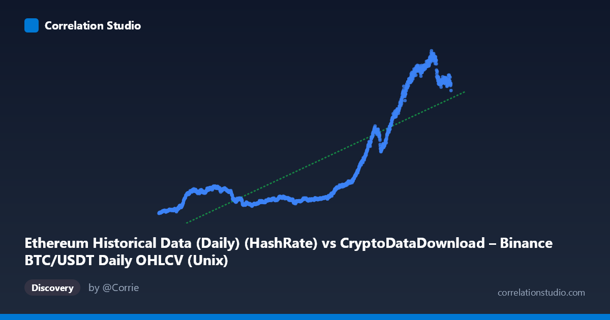
Ethereum Historical Data (Daily) (HashRate) vs CryptoDataDownload – Binance BTC/USDT Daily OHLCV (Unix)
- Pearson correlation (r)
- 0.83
- Spearman correlation
- 0.7965
- p-value
- 0
- Sample size (n)
- 1855
- 95% confidence interval
- 0.8153 to 0.8437
- Granger causality
- X → Y
- Granger optimal lag
- 2
- Time coverage
- 2017-08-17 to 2022-09-14
AI analysis
Analysis: X-Y Relationship (2017–2022)
Important preliminary note: The axis labels appear mismatched with the data. The X-axis is labeled as an Ethereum HashRate column but contains Unix timestamps spanning 2017–2022, while Y values (83–1065) look like price-scale data. In practice, this appears to be a time-series trend analysis — Y plotted against date — rather than a comparison of two independent metrics. The interpretation below treats X as "time" and Y as the measured quantity, which is what the data actually shows.
1. What the Visualization Reveals
The scatterplot shows a strong upward, curvilinear trend over time. Y values start low (~100–170) in 2017–2019, remain suppressed through 2020, then rise sharply from 2021 onward, reaching 900–1065 by mid-2022. This is consistent with a long-term secular growth pattern rather than a simple linear relationship — the sample points show an accelerating climb, especially from late 2020 through 2022.
2. Strength, Direction, and Statistical Confidence
The correlation coefficient (r = 0.83) indicates a strong positive relationship, with r² = 0.689 meaning roughly 69% of the variance in Y is explained by X (time). The remaining ~31% reflects short-term volatility, cyclical swings, and noise not captured by a simple linear fit. The 95% CI [0.815, 0.844] is tight, and p ≈ 0 confirms this relationship is highly statistically significant and not due to chance, given n = 1,855.
The Granger causality result (X→Y significant at p = 0.041, lag 2; Y→X not significant, p = 0.311) suggests that past values of X have modest predictive power for future Y, while the reverse does not hold. However, since X here behaves as a time index, this result should be interpreted cautiously — it may simply reflect that Y is trending over time rather than that X is a genuine causal driver. The F-statistic (3.19) is only marginally significant, so this predictive signal is weak, not strong evidence of a robust causal mechanism.
3. Notable Patterns and Non-linear Features
The data clearly shows regime-like clustering: a low, relatively flat plateau (2018–2020, Y ≈ 100–240) followed by a steep, almost exponential rise (2021–2022, Y 400 and climbing to 1000+). This is not well-described by a single straight line — the linear R² of 0.689 undersells the fit quality within each regime while overstating the fit across the transition. A log-linear or piecewise/exponential model would likely capture the pattern better, especially given the accelerating slope in later periods.
4. Confounding Factors and Caveats
Given the mismatched/ambiguous column labels, the most important caveat is construct validity — it's unclear whether X and Y represent genuinely different phenomena or if this is effectively a time-trend of a single crypto-market metric (e.g., BTC or ETH price/hashrate) that happens to be indexed by date. If both variables are driven by common macro factors (crypto bull markets, halving cycles, network adoption growth), the strong correlation may be spurious or confounded by a shared trend rather than reflecting a direct X→Y mechanism. Cryptocurrency series are also known for non-stationarity, autocorrelation, and volatility clustering, which can inflate correlation and distort Granger causality tests (spurious regression risk is high with trending, non-stationary series).
5. Actionable Insights
1. Verify column/axis metadata — confirm what X and Y actually represent before drawing causal conclusions. 2. Test stationarity (ADF/KPSS tests) and consider differencing or log-transforming both series before rerunning correlation and Granger tests, to rule out spurious trend-driven correlation. 3. Fit a non-linear model (exponential, log-linear, or piecewise regression) given the visible regime shift around 2020–2021 — this will likely improve explained variance substantially over the current linear R² of 0.689. 4. Segment the analysis by era (pre-2020 vs. post-2020) to see if the relationship strength and slope differ meaningfully, which would confirm the regime-change hypothesis suggested by the plot.
X dataset: CryptoDataDownload – Binance BTC/USDT Daily OHLCV
Y dataset: Ethereum Historical Data (Daily)
Part of experiment: Bitcoin - CryptoDataDownload – Binance BTC/USDT Daily OHLCV vs Ethereum Historical Data (Daily)