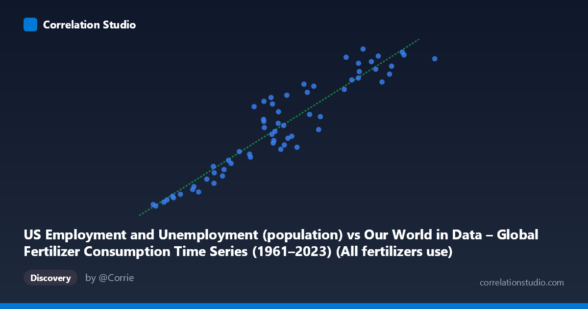
US Employment and Unemployment (population) vs Our World in Data – Global Fertilizer Consumption Time Series (1961–2023) (All fertilizers use)
- Pearson correlation (r)
- 0.9409
- Spearman correlation
- 0.9216
- p-value
- 0
- Sample size (n)
- 63
- 95% confidence interval
- 0.9038 to 0.9639
- Granger causality
- Y → X
- Granger optimal lag
- 10
- Time coverage
- 1961-01-01 to 2023-01-01
AI analysis
Analysis: US Employment Population vs. Global Fertilizer Consumption (1961–2023)
Relationship Overview The scatterplot reveals a strong, positive, approximately linear relationship between the US employment and unemployment population (X-axis) and global all-fertilizer consumption (Y-axis) across the 1961–2023 period. As the US employment population grows from roughly 3.2 million to 22.7 million units, global fertilizer consumption rises correspondingly from approximately 118,771 to 266,942 units. The data points track a reasonably tight upward trajectory, consistent with two variables that have both grown persistently over the same six-decade span. The linear regression equation (y = 0.00855x + 91,065) fits the cloud well visually, though some dispersion around the line is apparent at mid-range values.
Correlation Strength and Statistical Interpretation The Pearson correlation of r = 0.9409 is very high, and the R² of 0.8853 means that approximately 88.5% of the variance in global fertilizer consumption is statistically explained by variation in the US employment population within this sample. This is a remarkably high explanatory share for a simple bivariate model. The 95% confidence interval for r of [0.9038, 0.9639] is narrow and lies entirely in strongly positive territory, indicating low uncertainty about the direction and approximate magnitude of the association. The p-value of effectively zero confirms the result is not a chance artifact of sampling. However, the Granger causality results add an important temporal nuance: Y Granger-causes X (unidirectionally, at lag 10, F = 2.18, p = 0.046), meaning past values of global fertilizer consumption have statistically significant predictive power over future US employment population figures, but not vice versa (X→Y: p = 0.077, just above the 0.05 threshold). This is a counterintuitive direction if one were expecting US labor markets to drive agricultural input demand, and warrants careful interpretation.
Notable Patterns, Clusters, and Outliers The scatterplot shows a relatively clean linear sweep with no dramatic outliers, but several features are worth noting. The lower-left cluster (X ≈ 3–6 million, Y ≈ 118,000–135,000) represents earlier decades (1960s–1970s) where both series were at lower absolute levels. The upper-right cluster (X 18 million, Y 245,000) corresponds to more recent decades. A moderate band of scatter exists in the mid-range (X ≈ 10–14 million), where Y values span roughly 165,000–235,000 — a spread of ~70,000 units — suggesting that the relationship is somewhat looser in this zone and that other factors may introduce variability during this transitional period. No single point appears to be a severe leverage outlier, though the two extreme upper-right points (X ≈ 20.5–22.7 million) sit at the edge of the data cloud and could exert disproportionate influence on the regression slope.
Confounding Factors and Caveats The most critical caveat here is the classic spurious correlation driven by shared time trends. Both the US employment population and global fertilizer consumption have grown substantially and relatively monotonically since 1961, driven by independent underlying forces — US population growth, workforce participation trends, and economic expansion on one hand; global agricultural intensification, Green Revolution adoption, and population-driven food demand on the other. Two variables that both trend upward over 60 years will almost always produce high r and R² values, even if they have no mechanistic connection. The Granger causality direction (fertilizer consumption predicting US employment) makes little theoretical sense as a causal chain, reinforcing the suspicion that this is a shared-trend artifact rather than a meaningful predictive relationship. Additionally, the dataset labels appear to be swapped in axis attribution (the X-axis column is labeled from a fertilizer dataset, and Y from a US employment dataset), which introduces uncertainty about which variable is actually which, and warrants verification before any substantive conclusion is drawn.
Actionable Insights and Further Investigation Given the strong likelihood of spurious correlation, the most important next step is to detrend both series (e.g., using first differences or percentage year-on-year changes) and recompute the correlation — if r drops sharply toward zero, the relationship is almost certainly an artifact of shared temporal trends rather than any genuine co-movement. Researchers should also apply cointegration tests (e.g., Engle-Granger or Johansen) to determine whether the long-run relationship is statistically meaningful beyond shared trends. If a genuine link is hypothesized — for instance, that US agricultural labor inputs affect fertilizer demand, or vice versa — a theoretically grounded structural model with appropriate control variables (global population, food prices, GDP, policy shocks) would be needed. The Granger lag of 10 periods is also worth investigating: a decade-long lag between fertilizer consumption and US employment shifts has no obvious economic mechanism, suggesting the result may be a statistical artifact of autocorrelated series rather than a true predictive signal. Finally, correcting the apparent axis/dataset label mismatch should be the immediate first step before any further analysis proceeds.
X dataset: Our World in Data – Global Fertilizer Consumption Time Series (1961–2023)
Y dataset: US Employment and Unemployment
Part of experiment: Yearly - Our World in Data – Global Fertilizer Consumption Time Series (1961–2023) vs US Employment and Unemployment