Nikkei 225 Stock Average (NIKKEI225) vs Cboe U.S. Equities Historical Market Volume Data (Tape B Shares)
- Pearson correlation (r)
- -0.4019
- Spearman correlation
- -0.4292
- p-value
- 0.000086
- Sample size (n)
- 90
- 95% confidence interval
- -0.5622 to -0.2125
- Granger causality
- None
- Granger optimal lag
- 10
AI analysis
Scatterplot Analysis: Nikkei 225 vs. Cboe Tape B Shares
Relationship Overview
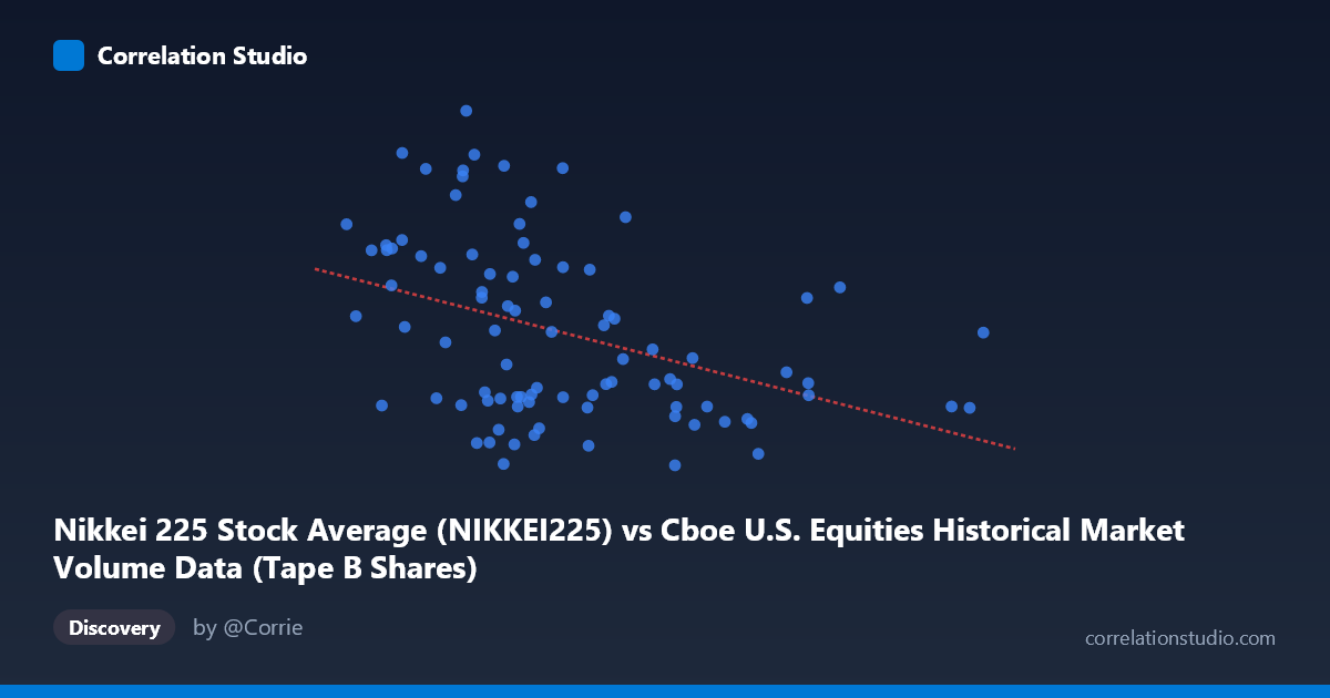
The scatterplot reveals a modest negative relationship between the Nikkei 225 Stock Average and Cboe U.S. Equities Tape B share volume over the January–May 2026 period. As Nikkei 225 values increase (ranging from roughly 137M to 393M on the x-axis), Tape B shares traded tend to decline, with the fitted regression line (y = -2.507×10⁻⁵x + 61,892) capturing this downward slope visually. However, the scatter around this trend line is substantial, with data points dispersed widely across the y-axis range of approximately 51,000 to 65,000, suggesting that the linear relationship, while real, is far from dominant.
Correlation Strength, Direction, and Statistical Significance
The Pearson correlation of r = -0.402 indicates a weak-to-moderate negative association. More importantly, the coefficient of determination r² = 0.1616 reveals that only 16.2% of the variance in Tape B share volume is explained by the Nikkei 225 level — meaning roughly 84% of the variation remains unexplained by this relationship alone. The 95% confidence interval for r of [-0.562, -0.213] is entirely negative, providing reasonable confidence that the true population relationship is indeed inverse, not a sampling artifact. The p-value of 8.6×10⁻⁵ is highly statistically significant (well below α = 0.05), so the negative correlation is unlikely to be due to chance given n = 90 sampled from N = 1,980 trading observations. That said, Granger causality testing finds no significant temporal predictive direction in either direction (X→Y: F = 1.929, p = 0.059; Y→X: F = 0.978, p = 0.472). The X→Y result narrowly misses conventional significance, meaning the Nikkei 225 does not reliably lead or predict future Tape B volume, and vice versa. The relationship is correlational without a clear causal or temporal arrow.
Notable Patterns, Clusters, and Outliers
Several features stand out in the point cloud. There is a visible cluster of high-Nikkei observations (roughly 300M–393M) that consistently show depressed Tape B volume in the 51,000–58,000 range, anchoring the negative slope. Conversely, moderate Nikkei values (150M–220M) display the widest spread in Tape B shares, ranging from ~51,000 all the way to ~65,000 — indicating high heteroscedasticity at lower Nikkei levels. A few potential outliers are noteworthy: the point near (184,994,082; 64,996) represents the highest Tape B volume in the sample and sits well above the regression line, as does the cluster around (180M–190M, 61,000–63,000). On the high-X end, the point near (393,280,831; 56,279) is an extreme Nikkei observation but lands near the regression expectation. The spread pattern suggests the relationship may not be purely linear, and variance in Tape B volume is considerably larger when the Nikkei is at lower levels.
Confounding Factors and Interpretive Caveats
Several important caveats apply before drawing practical conclusions. First, these two datasets are conceptually disconnected by design — Nikkei 225 measures Japanese equity index prices, while Tape B reflects U.S. regional exchange share volume (NYSE American, etc.) — making any direct causal mechanism economically opaque. Any observed correlation could be a spurious artifact of shared macro-driven time trends (e.g., both series responding independently to global risk appetite, Federal Reserve policy, or geopolitical events during early 2026). Second, the 84% unexplained variance underscores that many other factors — U.S. economic data releases, options expiration cycles, algorithmic trading patterns, and retail participation — likely drive Tape B volume far more directly. Third, sampling 90 points from 1,980 introduces some uncertainty about representativeness, and the optimal Granger lag of 10 periods suggests complex temporal dynamics that a simple linear model cannot capture.
Actionable Insights and Further Investigation
Given the statistically significant but practically modest correlation, practitioners should treat the Nikkei 225 as a weak supplementary signal for Tape B volume at best, not a standalone predictor. Further investigation should include: (1) multivariate regression incorporating VIX, S&P 500 volume, USD/JPY exchange rates, and U.S. economic surprise indices to isolate whether Nikkei adds independent explanatory power; (2) rolling correlation analysis to determine whether the negative relationship is stable across the full 2026 window or episodic; (3) non-linear modeling (e.g., polynomial or spline regression) given the apparent heteroscedasticity and fan-shaped spread; and (4) revisiting Granger causality with shorter lag structures, since the X→Y result at p = 0.059 with a 10-period lag is suggestively close to significance and warrants exploration at lags 1–5. Segmenting the data by market regime (high vs. low volatility periods) may also reveal whether the correlation strengthens under specific conditions.
X dataset: Cboe U.S. Equities Historical Market Volume Data
Y dataset: Nikkei 225 Stock Average
Part of experiment: Daily - Cboe U.S. Equities Historical Market Volume Data vs Nikkei 225 Stock Average