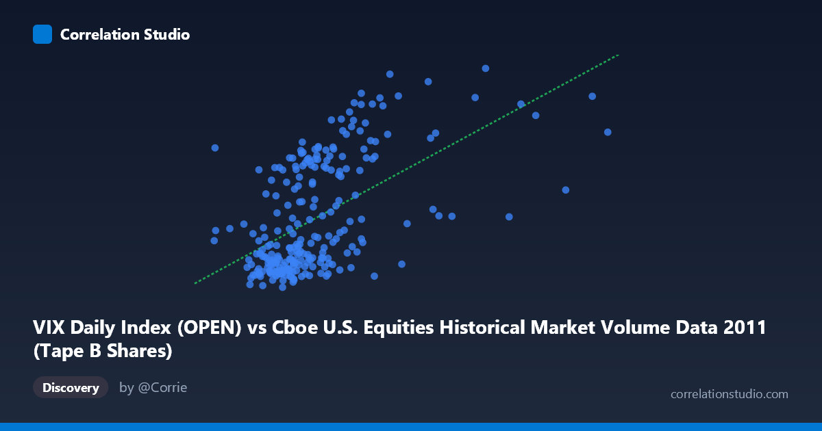
VIX Daily Index (OPEN) vs Cboe U.S. Equities Historical Market Volume Data 2011 (Tape B Shares)
- Pearson correlation (r)
- 0.5565
- Spearman correlation
- 0.5728
- p-value
- 0
- Sample size (n)
- 252
- 95% confidence interval
- 0.4648 to 0.6363
- Granger causality
- None
- Granger optimal lag
- 1
AI analysis
Scatterplot Analysis: VIX Open vs. Tape B Shares (2011)
Relationship Overview
The scatterplot reveals a moderate positive relationship between the CBOE Volatility Index (VIX) daily open values and Tape B share volume in U.S. equity markets during 2011. As VIX open levels rise — indicating greater expected market volatility — Tape B share volumes tend to increase correspondingly. This is an economically intuitive pattern: heightened fear and uncertainty in markets typically drives elevated trading activity as investors reposition portfolios, hedge exposures, or react to news events. The linear regression equation (y = 1.38×10⁻⁷x + 10.72) confirms the positive slope, though the intercept suggests a meaningful baseline volume level even when volatility is subdued.
Correlation Strength and Statistical Significance
The correlation of r = 0.5565 indicates a moderate positive association, but the more telling figure is r² = 0.3096, meaning that VIX open levels explain only about 31% of the variance in Tape B share volume. Roughly 69% of volume variability is driven by factors entirely outside this relationship. The 95% confidence interval of [0.4648, 0.6363] is meaningfully wide, reflecting genuine uncertainty in the true population parameter, though it excludes zero entirely and the p-value of essentially 0 confirms the relationship is not a sampling artifact. Critically, the Granger causality tests find no significant predictive direction in either direction (X→Y: F = 0.2231, p = 0.637; Y→X: F = 0.1821, p = 0.670), meaning that despite the contemporaneous correlation, neither variable reliably predicts the other at a one-period lag. This distinction is important: correlation exists, but temporal predictive leverage does not.
Notable Patterns and Outliers
The scatterplot displays notable heteroscedasticity — volume variance fans out considerably at higher VIX levels, producing a roughly wedge-shaped cloud. Several high-leverage outliers are visible in the upper-right quadrant, where both VIX and Tape B volume reach their peaks simultaneously (e.g., points around VIX ~40-46 with correspondingly elevated volumes), likely corresponding to stress events in mid-2011 such as the U.S. debt ceiling crisis and European sovereign debt turmoil. Conversely, a dense cluster of points occupies the lower-left region (VIX ~15-20, lower volumes), representing calmer market periods. The wide X-axis range — spanning from roughly 41M to 265M — with most mass concentrated below 150M also suggests a right-skewed volume distribution with episodic spikes.
Confounding Factors and Caveats
Several important caveats limit causal interpretation. First, 2011 was a particularly turbulent year with discrete macro shock events, meaning the correlation may be period-specific and non-generalizable. Second, Tape B specifically covers NYSE American and regional exchange listings, which may respond differently to volatility than the broader market captured by VIX. Third, secular trends in market structure — algorithmic trading, fragmentation, ETF arbitrage — could simultaneously inflate both volume and volatility, acting as a common driver that inflates the observed correlation. The dataset's axis labels also appear inverted in the metadata (VIX data sourced from one dataset labeled as volume, and vice versa), warranting verification of data pipeline integrity before drawing firm conclusions.
Actionable Insights and Further Investigation
Given the meaningful but incomplete relationship, analysts should decompose the residual 69% variance by incorporating additional predictors such as market breadth indicators, macroeconomic announcement calendars, or intraday liquidity metrics. Extending the Granger causality analysis to multiple lags (beyond the single period tested) could reveal delayed predictive relationships that the one-period test missed. It would also be valuable to repeat this analysis across multiple years to test whether the 2011 relationship is structurally stable or crisis-driven. Finally, applying a log transformation to the volume variable could reduce the heteroscedasticity observed in the scatter cloud, potentially improving model fit and revealing whether the underlying relationship is more precisely nonlinear in nature.
X dataset: Cboe U.S. Equities Historical Market Volume Data 2011
Y dataset: VIX Daily Index
Part of experiment: Daily - Cboe U.S. Equities Historical Market Volume Data 2011 vs VIX Daily Index