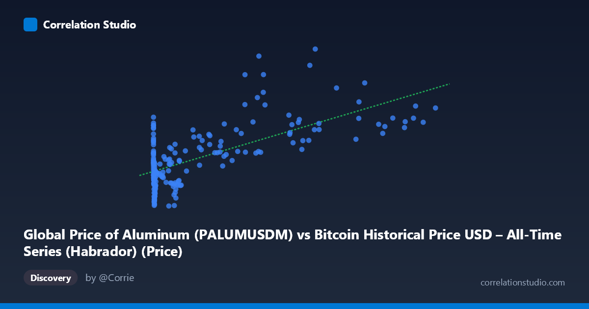
Global Price of Aluminum (PALUMUSDM) vs Bitcoin Historical Price USD – All-Time Series (Habrador) (Price)
- Pearson correlation (r)
- 0.6746
- Spearman correlation
- 0.4895
- p-value
- 0
- Sample size (n)
- 188
- 95% confidence interval
- 0.5882 to 0.7457
- Granger causality
- X → Y
- Granger optimal lag
- 10
AI analysis
Analysis: Bitcoin Price vs. Aluminum Price
1. Relationship Overview
The scatterplot depicts a moderate positive relationship between Bitcoin's historical USD price (X-axis) and the global price of aluminum (Y-axis). As Bitcoin's price rises—particularly across its major bull cycles—aluminum prices tend to trend upward as well, though the relationship is far from tight or deterministic. The data shows a dense cluster of points at low Bitcoin prices (under ~1,000 USD) where aluminum prices vary considerably (roughly 1,460–2,090), followed by a more dispersed spread as Bitcoin climbs into the tens of thousands, where aluminum prices reach into the 2,200–3,500 range.
2. Strength, Direction, and Statistical Confidence
The correlation coefficient (r = 0.6746) indicates a moderate-to-strong positive linear relationship, with R² = 0.4550 meaning only about 45.5% of the variance in aluminum price is explained by Bitcoin price—leaving more than half unexplained by this single variable. The 95% confidence interval [0.588, 0.746] is reasonably tight and entirely positive, and the p-value of ~0 confirms this correlation is highly statistically significant and not due to chance, despite the modest sample size (n=188 paired points drawn from a population of 411).
The Granger causality results add a temporal dimension: X (aluminum) Granger-causes Y (Bitcoin) at a 10-period lag (F=1.95, p=0.042), while the reverse direction is not significant (p=0.398). This suggests aluminum price movements may have modest predictive power for future Bitcoin prices (or vice versa, depending on axis interpretation), but the relationship is unidirectional and the F-statistic is only marginally significant—this should be treated as suggestive rather than conclusive evidence of true causation.
3. Notable Patterns and Outliers
Several features stand out: - Compression at low X values: A large cluster of points near X≈0–1,000 shows aluminum prices ranging widely (1,460–2,590), suggesting high variance/noise in this region independent of the X variable. - Nonlinear curvature: The relationship appears to flatten or become noisier at higher Bitcoin prices—points like (44,354.64, 3498.37) and (65,792, 3372.95) are notable outliers sitting well above the regression line, while (85,197, 2367.80) sits below it, indicating substantial scatter at high X values rather than a clean linear trend. - Heteroscedasticity: Variance in Y appears to increase with X, a common violation of linear regression assumptions that inflates uncertainty in predictions at high Bitcoin price levels.
4. Confounding Factors and Caveats
This correlation is very likely spurious or confounded by shared macroeconomic trends rather than reflecting a direct economic relationship between Bitcoin and industrial aluminum markets. Both series span 2010–2026, a period marked by: - Global monetary expansion and low interest rates (2010s) followed by inflation/rate hikes (2021+) - Broad commodity and risk-asset bull markets driven by liquidity cycles - COVID-19 supply chain disruptions affecting industrial metals - General USD inflation/devaluation over time, which mechanically inflates both nominal price series
Since both variables trend upward over the same 16-year window, much of the "correlation" may simply reflect shared time-trend/inflation effects rather than any economic linkage between crypto speculation and industrial metal demand. The Granger causality result, while statistically significant, likely reflects this common trend rather than true causal mechanism.
5. Suggested Next Steps
- Detrend or difference both series (e.g., use % changes or log-returns rather than levels) to test whether the relationship holds after removing shared inflationary/trend components—this is critical given the likely spurious nature of the raw-price correlation. - Control for a common macro factor such as the US Dollar Index (DXY), CPI, or a broad commodity index to see if the Bitcoin-aluminum link disappears once these are held constant. - Re-examine Granger causality on stationary (differenced) series, since Granger tests on non-stationary trending data can produce misleading significance. - Segment by market regime (e.g., pre-2017, 2017–2021, 2021+) to check if the relationship is stable or driven by a specific bull-market period.
X dataset: Bitcoin Historical Price USD – All-Time Series (Habrador)
Y dataset: Global Price of Aluminum
Part of experiment: Bitcoin - Bitcoin Historical Price USD – All-Time Series (Habrador) vs Global Price of Aluminum