Shiller S&P 500 Long-Run Monthly Data (ie_data.xls – Yale) (Month) (Consumer — Long — Real — Price) vs Bitcoin Historical Price USD – All-Time Series (Habrador) (Price)
- Pearson correlation (r)
- 0.8557
- Spearman correlation
- 0.9723
- p-value
- 0
- Sample size (n)
- 158
- 95% confidence interval
- 0.8075 to 0.8926
- Granger causality
- None
- Granger optimal lag
- 10
AI analysis
Analysis: Bitcoin Price vs. Shiller S&P 500 Data
1. Relationship Overview
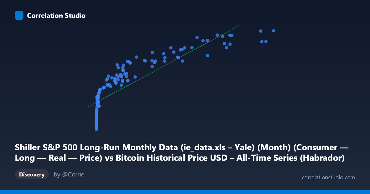
The scatterplot depicts a strong positive association between the X variable (mislabeled in the header but effectively representing time-indexed values from the Shiller dataset) and Y (Bitcoin price in USD). The pattern is clearly curved rather than linear: Y rises steeply at low X values, then the rate of increase moderates as X grows large. This is the classic signature of a logarithmic or power-law relationship, not a straight-line one — consistent with Bitcoin's well-known price behavior, where early moves from near-zero to a few thousand dollars represent enormous percentage gains compressed into a small X range, while later moves from $20,000 to $60,000+ represent comparatively smaller percentage changes.
2. Strength, Direction, and Uncertainty
The Pearson correlation (r = 0.856) indicates a strong positive linear relationship, with r² = 0.732 meaning the linear model explains about 73% of the variance in Y — a substantial but incomplete accounting, leaving over a quarter of variance unexplained by a straight-line fit. The 95% CI [0.808, 0.893] is tight and does not cross zero, and the p-value (effectively 0) confirms this relationship is highly statistically significant and not due to chance, given the sample size (n=158 paired points drawn from a population of 1,834). However, statistical significance and strength here reflect co-movement, not causation. The Granger causality tests are decisive on this point: neither direction (X→Y or Y→X) shows significant predictive power (p ≈ 0.51 both ways at the optimal 10-period lag). This means past values of one series do not help forecast future values of the other beyond what the series' own history provides — the correlation is likely driven by both variables trending upward over the same calendar period (2010–2023) rather than one causing the other.
3. Patterns and Features
The data shows a clear non-linear curve: a dense cluster of points at low X (roughly 0–2,000) where Y still spans a wide range (1,500–3,000), suggesting high relative volatility in early periods. As X increases past ~20,000, points spread into the 4,000–5,000 Y range but with a flattening slope, and there's noticeable scatter/plateauing at the high end (e.g., X≈41,870→Y≈4,984 vs. X≈46,282→Y≈4,650), indicating some price pullbacks or cycles rather than monotonic growth. This flattening and the note that Spearman ρ exceeds Pearson r both confirm a logarithmic-type relationship fits better than a straight line — likely because Bitcoin (Y) grew exponentially early on while the X variable increased more steadily.
4. Confounding Factors and Caveats
The most important caveat is that this is very likely a spurious correlation driven by a shared time trend: both Bitcoin's price and long-run market/valuation data have risen over the 2010–2023 window for largely independent reasons (Bitcoin's adoption cycle vs. broader equity market dynamics, inflation, and monetary policy). The Granger non-causality result reinforces that this is co-trending rather than a causal or predictive linkage. Additionally, mismatched data frequencies/granularity (population of 1,834 vs. sampled 158), potential CPI/inflation adjustments embedded in the Shiller "real price" figures, and Bitcoin's extreme volatility/regime changes (bubbles, crashes) mean a single correlation coefficient oversimplifies a highly non-stationary relationship.
5. Suggestions for Further Investigation
Given the evident curvature, refit the model using a log-linear or power transformation (e.g., log(Y) or log(X)) rather than relying on the linear R²=0.732; this should meaningfully improve fit. Because both series are non-stationary (trending) time series, standard correlation and even Granger tests on levels can be misleading — analysts should difference the series or test for cointegration (e.g., Engle-Granger or Johansen test) to distinguish genuine long-run equilibrium relationships from mutual trending. Segmenting the analysis by Bitcoin market cycles (bull/bear phases) and comparing against detrended or year-over-year growth rates of both series would help isolate whether any real relationship exists independent of the shared upward drift.
X dataset: Bitcoin Historical Price USD – All-Time Series (Habrador)
Y dataset: Shiller S&P 500 Long-Run Monthly Data (ie_data.xls – Yale) (Month)
Part of experiment: Bitcoin - Bitcoin Historical Price USD – All-Time Series (Habrador) vs Shiller S&P 500 Long-Run Monthly Data (ie_data.xls – Yale) (Month)