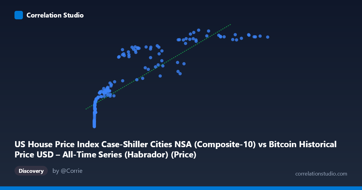
US House Price Index Case-Shiller Cities NSA (Composite-10) vs Bitcoin Historical Price USD – All-Time Series (Habrador) (Price)
- Pearson correlation (r)
- 0.8543
- Spearman correlation
- 0.9702
- p-value
- 0
- Sample size (n)
- 187
- 95% confidence interval
- 0.8101 to 0.8888
- Granger causality
- None
- Granger optimal lag
- 9
AI analysis
Analysis: Bitcoin Price vs. US Case-Shiller Home Price Index
1. Relationship Overview
The scatterplot shows a strong, clearly non-linear positive relationship between Bitcoin price (X) and the Case-Shiller Home Price Index (Y). At low Bitcoin values (roughly $0–$1,000), Y compresses tightly into a narrow band (~146–210), then rises steeply as X increases into the tens of thousands, before flattening again as Bitcoin approaches its historical highs (Y plateaus near 350–363). This produces a classic logarithmic or saturating-curve shape rather than a straight line — consistent with the note that Spearman's ρ exceeds Pearson's r.
2. Strength, Direction, and Statistical Confidence
The Pearson correlation (r = 0.854) is strong and positive, with r² indicating that a linear model explains about 73% of the variance in Y. The 95% CI [0.810, 0.889] is tight and does not cross zero, and the p-value is effectively 0, so the linear association is statistically robust and not a artifact of sampling noise. However, correlation here should not be read as causation: the Granger causality tests (lag=9) show no significant predictive direction in either direction (X→Y: p=0.77; Y→X: p=0.81). This means neither series helps forecast the other's future values based on past values — the strong contemporaneous correlation likely reflects both series trending upward over the same historical period (2010–2026) rather than one driving the other.
3. Notable Patterns and Features
- Curvature: The relationship is concave/logarithmic — early Bitcoin growth (pennies to thousands) corresponds to modest home-price movement, while the steep-growth non-linear zone occurs between roughly $5,000–$60,000, and further BTC gains beyond ~$80,000 correspond to diminishing Y increases (index approaching a ceiling near 360). - Clustering: A dense cluster of low-X points (X < 1,000) all map to Y values between 146–213, suggesting the model has little discriminating power in this range. - Plateau outliers: Points like (44,354 → 317.75) vs. (105,620 → 362.82) show some scatter/non-monotonicity at high X, indicating the relationship isn't perfectly smooth at the top end — likely reflecting Bitcoin's high volatility (crashes/rallies) against a comparatively stable housing index.
4. Confounding Factors and Caveats
Both series are essentially time trends — Bitcoin price and US home prices have both risen substantially since 2010–2011, largely independently, driven by very different macro forces (crypto adoption/speculation vs. housing supply, interest rates, demographics). This shared upward drift over 15+ years is a classic case of spurious correlation via a common time trend, rather than genuine economic linkage. The mismatched "n" (187) vs. population (470) suggests aggregation or resampling (e.g., converting daily BTC data to match monthly HPI data), which can smooth out volatility and inflate apparent correlation. Additionally, using raw (non-detrended) price levels for both variables violates stationarity assumptions of correlation analysis — this should ideally be done on returns/log-differences.
5. Suggestions for Further Investigation
- Detrend and test returns: Re-run correlation/Granger analysis on log-returns or first differences of both series to strip out the shared trend and see if any genuine short-term co-movement exists. - Fit non-linear models: Given the note on Spearman Pearson, try a log-transform of X (log(BTC price)) against Y, or a polynomial/logistic curve, which should meaningfully improve fit over the current linear R²=0.73. - Control for macro variables: Introduce interest rates, inflation, or a general stock market index (S&P 500) as covariates to test whether both series are merely correlated with broader macroeconomic liquidity/risk-on conditions. - Treat correlation as descriptive only: Given the null Granger result, avoid using Bitcoin price as a leading indicator for housing prices (or vice versa) in any forecasting model; the relationship appears coincidental/trend-driven rather than causal or predictive.
X dataset: Bitcoin Historical Price USD – All-Time Series (Habrador)
Y dataset: US House Price Index Case-Shiller Cities NSA
Part of experiment: Bitcoin - Bitcoin Historical Price USD – All-Time Series (Habrador) vs US House Price Index Case-Shiller Cities NSA