World Bank CO2 Emissions by Country (DataBank) (Total) vs US Employment and Unemployment (nonagriculture_ratio)
- Pearson correlation (r)
- 0.9427
- Spearman correlation
- 0.9313
- p-value
- 0
- Sample size (n)
- 80
- 95% confidence interval
- 0.9119 to 0.963
- Granger causality
- None
- Granger optimal lag
- 10
AI analysis
Scatterplot Analysis: World Bank CO2 Emissions vs. US Non-Agriculture Employment Ratio
Relationship Overview
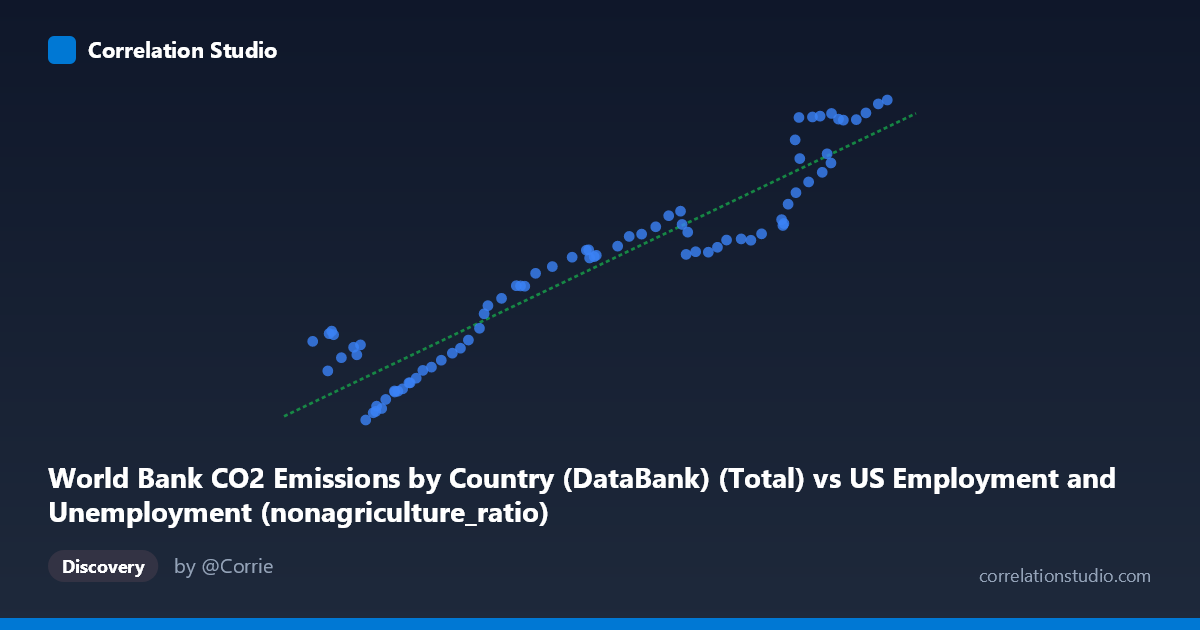
The scatterplot reveals a strong positive relationship between total CO2 emissions (X-axis) and the US non-agriculture employment ratio (Y-axis) spanning eight decades from 1941 to 2020. As CO2 emissions increase from approximately 41,250 to 155,113 units, the non-agriculture employment ratio rises correspondingly from roughly 9,870 to 43,129. The linear regression model (y = 0.2514x + 1,312) fits the data reasonably well across much of the range, suggesting that both variables have trended upward together over the long arc of the 20th and early 21st centuries — almost certainly reflecting their shared dependence on underlying economic and industrial growth rather than any direct causal mechanism between them.
Correlation Strength and Statistical Interpretation
The Pearson correlation of r = 0.9427 is exceptionally strong, and the coefficient of determination r² = 0.8888 indicates that approximately 88.9% of the variance in the non-agriculture employment ratio is statistically explained by variation in CO2 emissions within this sample. The 95% confidence interval of [0.9119, 0.9630] is narrow and lies entirely in the strongly positive region, confirming high precision in the estimate. The p-value of effectively zero (p ≈ 0) rules out the possibility that this correlation arose by chance across the n = 80 paired observations. However, the Granger causality results critically temper any causal interpretation: neither direction (X→Y: F = 0.895, p = 0.545; Y→X: F = 0.893, p = 0.546) achieves statistical significance at optimal lag 10, meaning neither variable temporally predicts the other beyond what each already predicts from its own past values. This strongly suggests the correlation is spurious or driven by a common third factor — most likely long-run economic expansion — rather than reflecting any meaningful directional influence.
Notable Patterns, Clusters, and Outliers
Several features depart from a clean linear relationship and deserve attention. A distinct cluster of points in the upper-right region (X ~135,000, Y ~40,000) appears to deviate slightly above the regression line, suggesting the relationship may steepen or plateau at high emission levels — possibly indicating a non-linear or saturation dynamic in later decades. Conversely, a cluster of lower-left points (X < ~65,000, Y < ~16,000) shows some scatter around the line, with a few notable outliers: the point near (41,250, 18,044) and (44,500, 18,843) sit conspicuously above the regression line for their X values, suggesting these early years had higher non-agriculture ratios than emissions alone would predict. Similarly, (51,758, 9,870) falls below the trend, indicating an unusually low employment ratio relative to its emission level. These anomalies likely reflect wartime and immediate post-war labor market disruptions of the early 1940s, where structural employment patterns did not yet track the industrialization trajectory.
Confounding Factors and Interpretation Caveats
This correlation is a textbook example of spurious correlation driven by shared secular trends. Both variables — total (likely global or US) CO2 emissions and US non-agriculture employment — have grown monotonically over most of the 20th century, driven by population growth, GDP expansion, industrialization, and post-war economic development. Any two variables sharing a long-run upward trend will naturally correlate strongly in time-series analysis without implying any real connection. Additional caveats include: (1) the X-axis label ambiguity — the dataset is described as "World Bank CO2 by Country" but the column appears in a US employment dataset, raising questions about whether this represents US-only or global emissions; (2) the label inversion between axes and dataset descriptions warrants careful verification before drawing conclusions; (3) the optimal Granger lag of 10 periods is relatively long, and the non-significance may reflect insufficient statistical power or structural breaks rather than a true absence of temporal dynamics; and (4) the data span includes major structural disruptions (WWII, oil crises, 2008 recession, COVID-19) that could introduce regime-dependent behavior masked by the aggregate trend.
Actionable Insights and Further Investigation
Given the absence of Granger causality and the likely spurious nature of the correlation, the immediate practical insight is to avoid policy or causal inference based on this association alone. For deeper investigation, analysts should: (1) detrend both series (e.g., using first differences or HP filtering) to remove the shared secular trend and retest correlation on residuals, which would reveal whether any relationship persists beyond common growth; (2) introduce GDP or industrial output as a control variable to test whether it fully mediates the association; (3) segment the analysis by decade to determine whether the relationship is stable across time or driven disproportionately by specific eras; (4) investigate the upper-right cluster separately, as the post-2000 data points may reflect a decoupling dynamic (e.g., if US emissions plateau while employment continues shifting toward services); and (5) clarify the geographic scope of the CO2 variable, since a global total paired with a US domestic labor metric introduces additional conceptual misalignment that could distort interpretation.
X dataset: US Employment and Unemployment
Y dataset: World Bank CO2 Emissions by Country (DataBank)
Part of experiment: Yearly - US Employment and Unemployment vs World Bank CO2 Emissions by Country (DataBank)