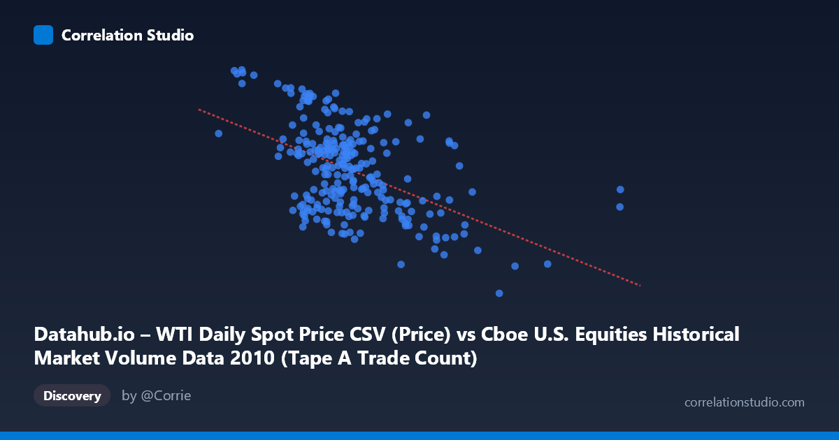
Datahub.io – WTI Daily Spot Price CSV (Price) vs Cboe U.S. Equities Historical Market Volume Data 2010 (Tape A Trade Count)
- Pearson correlation (r)
- -0.4967
- Spearman correlation
- -0.4199
- p-value
- 0
- Sample size (n)
- 252
- 95% confidence interval
- -0.5844 to -0.3975
- Granger causality
- None
- Granger optimal lag
- 1
AI analysis
Scatterplot Analysis: WTI Oil Price vs. Tape A Trade Count (2010)
Relationship Overview
The scatterplot reveals a moderate negative relationship between WTI crude oil daily spot prices (X-axis) and Cboe Tape A trade counts (Y-axis) across 2010 U.S. equity market trading days. As oil prices rise, the number of equity trades on Tape A venues tends to decline. The linear regression equation (y = -6.74×10⁻⁶x + 88.35) confirms this inverse slope, though the wide scatter around the regression line makes clear this is a noisy, imperfect relationship rather than a tight coupling. Visually, the data cloud slopes downward from left to right, but with substantial vertical dispersion at nearly every price level, suggesting many other forces are simultaneously shaping trade count activity.
Correlation Strength and Statistical Significance
The Pearson correlation of r = -0.497 indicates a moderate negative association, but the variance explained metric tells a more sobering story: r² = 0.247, meaning WTI oil prices account for only about 24.7% of the variance in Tape A trade counts, leaving roughly 75% unexplained by this single variable. The 95% confidence interval of [-0.584, -0.398] is meaningfully away from zero and relatively tight given the sample size (n = 252), lending credibility to the direction of the effect. The p-value of effectively zero confirms the correlation is statistically significant and very unlikely to be a sampling artifact. However, Granger causality testing complicates the narrative considerably — neither direction shows significant temporal predictive power at conventional thresholds (X→Y: F = 0.81, p = 0.370; Y→X: F = 3.65, p = 0.057). This strongly suggests that while the two variables co-move statistically, oil prices do not reliably predict future trade counts, nor vice versa — the correlation may be driven by shared underlying forces rather than any direct causal mechanism.
Notable Patterns, Clusters, and Outliers
Several features stand out in the sample points. At lower X values (roughly 600,000–1,000,000 range), trade counts cluster toward the higher end (85–91), consistent with the negative trend, and points like (627,720, 90.84) and (796,428, 89.83) anchor the upper-left region. Conversely, high-X outliers such as (3,216,587, 75.10) and (2,474,888, 68.03) sit in the lower-right, reinforcing the downward slope. There are also notable within-cluster anomalies — for instance, (1,024,361, 88.66) and (888,899, 89.33) show high trade counts at moderate X values, while (1,668,735, 68.23) and (1,631,831, 82.89) at similar X values diverge by nearly 15 units in Y, suggesting high local variability. The data do not exhibit an obviously non-linear (e.g., U-shaped or exponential) pattern, though the variance in Y appears somewhat larger in the mid-range of X than at the extremes, hinting at possible heteroscedasticity.
Confounding Factors and Interpretive Caveats
This correlation almost certainly reflects shared exposure to broader macroeconomic conditions in 2010 rather than a direct causal link. The year 2010 was characterized by post-financial-crisis recovery, elevated volatility episodes, and macroeconomic uncertainty (e.g., European sovereign debt concerns, Fed policy shifts). During periods of economic anxiety, risk-off sentiment might simultaneously depress oil prices and reduce equity trading activity, while recoveries could drive oil higher as equity volumes normalize — or vice versa, depending on the episode. Additionally, the dataset axes appear to be swapped in labeling (price data attributed to a volume dataset and trade counts attributed to a price dataset), which introduces metadata ambiguity that should be verified before drawing firm conclusions. The Granger causality near-miss (Y→X: p = 0.057) is worth noting — with a slightly more permissive threshold or a larger lag window, there could be a marginal signal worth revisiting.
Actionable Insights and Further Investigation
Given that oil prices explain only ~25% of trade count variance and show no significant Granger causality, practitioners should not use WTI prices alone as a trading volume predictor. More productive next steps would include: (1) adding control variables such as VIX (volatility index), S&P 500 returns, and Fed announcement dates to build a multivariate model that better captures the remaining ~75% of variance; (2) extending the time horizon beyond 2010 to test whether the negative correlation is a structural feature or a regime-specific artifact of post-crisis dynamics; (3) testing non-linear models (e.g., spline regression or quantile regression) to check whether the relationship strengthens or changes character at price extremes; and (4) re-examining the Granger causality at longer lags (5–10 periods) since market participants may respond to sustained oil price trends rather than single-day moves. The correlation is real but contextually thin — treat it as a hypothesis-generating finding rather than an operational signal.
X dataset: Cboe U.S. Equities Historical Market Volume Data 2010
Y dataset: Datahub.io – WTI Daily Spot Price CSV
Part of experiment: Daily - Cboe U.S. Equities Historical Market Volume Data 2010 vs Datahub.io – WTI Daily Spot Price CSV