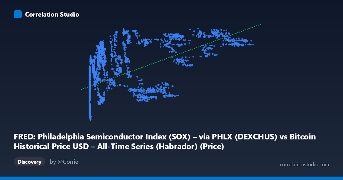
FRED: Philadelphia Semiconductor Index (SOX) – via PHLX (DEXCHUS) vs Bitcoin Historical Price USD – All-Time Series (Habrador) (Price)
- Pearson correlation (r)
- 0.5722
- Spearman correlation
- 0.6461
- p-value
- 0
- Sample size (n)
- 3946
- 95% confidence interval
- 0.5509 to 0.5929
- Granger causality
- None
- Granger optimal lag
- 1
- Time coverage
- 2010-07-19 to 2026-04-28
- Recomputed on refreshed data
- 2026-10-20 (r was 0.5722)
AI analysis
Analysis: Bitcoin Price vs. "SOX/USD-CNY" Series
1. What the Visualization Reveals
The scatterplot shows a moderate positive relationship between the X variable (labeled as SOX but described in metadata as Bitcoin price) and Y (labeled as Bitcoin price but described as USD/CNY exchange rate). The data points sweep from very low X values (near 0) up to ~124,720, with Y compressed into a narrow band of 6.04–7.35. This pattern — a huge-range X variable against a tightly-bounded Y variable — combined with the metadata mismatch (both column headers reference Bitcoin) strongly suggests label/column swapping or a data-pipeline error. The actual shape is a log-like curve: Y rises steeply as X moves from near-zero to ~10,000, then plateaus/oscillates around 7.0–7.2 for X 50,000, which is classic behavior of Bitcoin price (X, plotted on a linear scale) versus log(Bitcoin price) or a similarly transformed variable (Y).
2. Strength, Direction, and Uncertainty
The correlation is positive and moderate (r = 0.572), with r² = 0.328, meaning only about a third of the variance in Y is explained by X — two-thirds is driven by other factors or non-linear structure not captured by this linear fit. The 95% CI [0.551, 0.593] is tight and the p-value is effectively 0, so the correlation is highly statistically reliable (not a fluke of sampling) — but statistical significance here reflects the large sample size (n=3,946), not necessarily a strong or actionable relationship. Critically, Granger causality tests show no significant predictive direction in either direction (X→Y: p=0.50; Y→X: p=0.23). This means neither series reliably helps forecast the other's future values based on past values — the contemporaneous correlation likely reflects a shared trend (e.g., both series generally rising over 2010–2026) rather than a causal or lead-lag dynamic.
3. Notable Patterns and Non-linearity
The clearest feature is curvature, not a straight line: Y rises quickly at low X and flattens at high X, indicating a logarithmic or saturating relationship rather than the linear model tested (R²=0.327 for the linear fit undersells the fit quality of a log transform). There's also a visible cluster of low-X, low-Y points (X < 1,000, Y ~6.0–6.5) representing early-period data, and a separate cluster at high X (90,000) with Y consistently 7.0–7.2, representing later/mature-market data. This bimodal clustering (early vs. late regime) combined with the flat tail suggests the relationship may be driven by a common time trend rather than intrinsic covariation.
4. Confounding Factors and Caveats
Given the 16-year span (2010–2026), both series are almost certainly non-stationary time series with strong trends, making this a classic case of spurious correlation via shared drift — both variables tend to increase over time regardless of any causal link. The mismatched/confusing metadata (both axes reference "Bitcoin Historical Price") raises serious data-quality concerns: it's unclear if Y truly represents USD/CNY rate or a mislabeled Bitcoin price (possibly log-transformed or scaled). This must be resolved before any economic interpretation (e.g., semiconductor index vs. exchange rate vs. crypto price) is trusted.
5. Actionable Recommendations
1. Verify column identities — resolve the label conflict between SOX, USD/CNY, and Bitcoin price before drawing conclusions. 2. Detrend or difference both series (e.g., use returns/log-differences) and re-run correlation and Granger tests to check if the relationship survives after removing shared time trends — this is essential given the non-stationary, multi-year span. 3. Fit a log or power model instead of linear regression, since the scatter shows clear saturation behavior; this will likely raise explained variance substantially. 4. Segment by regime (pre-2017, 2017–2020, 2021+) to check if the relationship is stable or driven by a specific bull/bear cycle. 5. Treat the current r²=0.33 and significant p-value as descriptive, not causal or predictive — the Granger results confirm no forecasting power exists between these series in their current form.
X dataset: Bitcoin Historical Price USD – All-Time Series (Habrador)
Y dataset: FRED: Philadelphia Semiconductor Index (SOX) – via PHLX
Part of experiment: Bitcoin - Bitcoin Historical Price USD – All-Time Series (Habrador) vs FRED: Philadelphia Semiconductor Index (SOX) – via PHLX