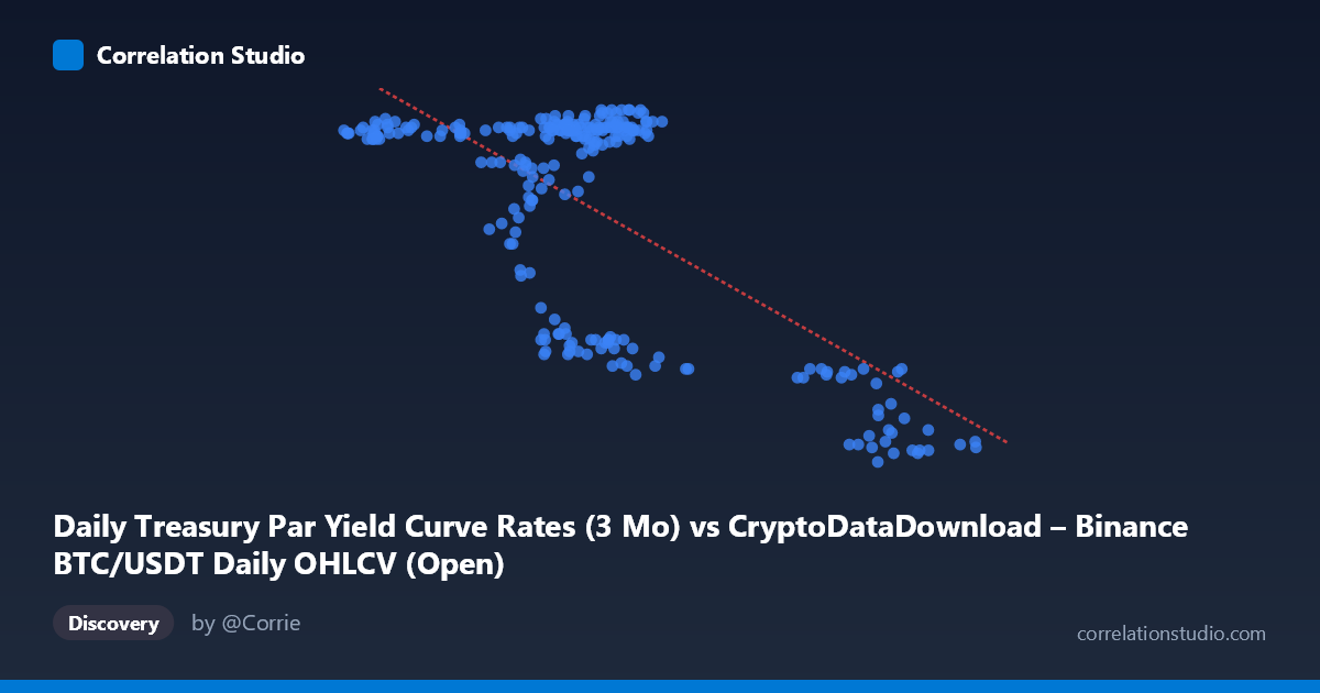
Daily Treasury Par Yield Curve Rates (3 Mo) vs CryptoDataDownload – Binance BTC/USDT Daily OHLCV (Open)
- Pearson correlation (r)
- -0.6905
- Spearman correlation
- -0.3136
- p-value
- 0
- Sample size (n)
- 250
- 95% confidence interval
- -0.7503 to -0.6195
- Granger causality
- None
- Granger optimal lag
- 1
- Time coverage
- 2024-01-02 to 2024-12-31
AI analysis
Analysis: Treasury 3-Month Yield vs. BTC/USDT Open Price
1. Relationship Overview
The scatterplot reveals a moderate-to-strong negative relationship between the two variables. As the "X" values (labeled Treasury Par Yield but populated with what appear to be BTC/USDT price-like magnitudes, ranging ~39,568–106,134) increase, the "Y" values (ranging 4.31–5.52) tend to decrease. The data does not form a simple linear cloud but instead shows a distinct clustering pattern: a dense group of points where X is roughly 40,000–70,000 and Y sits high (~5.2–5.5), and a second, sparser cluster where X exceeds ~90,000 and Y drops sharply to ~4.3–4.6. This bimodal clustering suggests the relationship may be better characterized as a regime shift rather than a smooth continuous decline.
2. Strength, Direction, and Statistical Confidence
The Pearson correlation of r = -0.6905 indicates a moderately strong negative linear association. The r² value of 0.4768 means only about 47.7% of the variance in Y is explained by X — leaving more than half of the variability unaccounted for by this simple linear relationship. The 95% confidence interval [-0.7503, -0.6195] is reasonably tight and does not cross zero, and the p-value of ~0 confirms this correlation is highly statistically significant and not due to chance, given the sample size of 250. However, statistical significance should not be conflated with strong predictive power — the moderate r² leaves substantial room for other factors. Critically, the Granger causality tests show no significant predictive direction in either direction (X→Y: p=0.33; Y→X: p=0.37). This means that despite the contemporaneous correlation, neither series helps forecast the other's future values based on past values — the relationship is associative, not (Granger-)causal or temporally predictive.
3. Notable Patterns and Outliers
The most striking feature is the two-cluster structure rather than a continuous linear trend. The main cluster (X≈40,000–71,000) shows high, relatively stable Y values with a secondary sub-band around Y≈4.6–4.7 at X≈58,000–70,000, suggesting a possible transitional or mixed regime. The second cluster (X≈90,000–106,000) shows uniformly low Y values (~4.3–4.6) with much less spread. This suggests a threshold or non-linear step-like relationship — Y stays relatively high and variable until X crosses roughly 70,000–90,000, after which Y drops and stabilizes at a lower level. This pattern is more consistent with a regime-based/non-linear relationship than the linear model implies, meaning the linear r² may understate or mischaracterize the true relationship structure.
4. Confounding Factors and Caveats
Several caveats are important. First, the metadata is confusing/contradictory: the X-axis is labeled as Treasury 3-Month yield but described as sourced from BTC/USDT OHLCV, while Y is labeled as BTC/USDT Open but sourced from Treasury yield data — this labeling mismatch should be resolved before drawing economic conclusions. Second, both series are time-based (2024 daily data), so autocorrelation within each series (trending, non-stationarity) can inflate cross-correlation without implying genuine relationship — this is a classic spurious correlation risk with financial/macro time series. Third, the clustering pattern suggests a confound such as a shared time trend or a small number of discrete "regime" days (e.g., a period of high X coinciding with a policy shift or market event) rather than a continuous causal mechanism. Finally, with only 250 points across a single year, seasonal effects, macro events, or a handful of extreme days could disproportionately drive the correlation.
5. Recommendations for Further Investigation
To clarify the true relationship, analysts should: (1) verify and correct the axis/column labeling to ensure the variables are correctly identified; (2) test for stationarity (e.g., ADF test) and consider differencing or detrending both series before correlating, since non-stationary series often produce misleadingly high correlations; (3) explore non-linear or piecewise/threshold regression models given the apparent two-cluster structure; (4) segment the data by date to see if the clusters correspond to distinct calendar periods (e.g., early vs. late 2024) rather than a smooth functional relationship; and (5) given the null Granger causality result, avoid using one series to forecast the other — instead treat the correlation as descriptive/contemporaneous only, and investigate potential common external drivers (e.g., macroeconomic conditions, Fed policy, risk sentiment) that could simultaneously affect both series.
X dataset: CryptoDataDownload – Binance BTC/USDT Daily OHLCV
Y dataset: Daily Treasury Par Yield Curve Rates
Part of experiment: Bitcoin - CryptoDataDownload – Binance BTC/USDT Daily OHLCV vs Daily Treasury Par Yield Curve Rates